Continuous Profiling on AWS - Which Clock the Flame Graph Is Showing You, What Runtime Metrics Cannot Replace, and What Sampling Never Sees

First Published: 2026-09-08
Last Updated: 2026-09-08

The traces are already in place. The service map has identified the slow node, and the span waterfall has pinpointed the single call that is consuming the time. That much is done.

And then it stops.

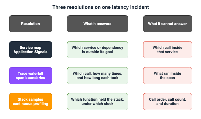
The traces do not know what happens inside those spans. They only record the start time, the end time, and whatever attributes were attached to them. The traces do not distinguish between whether that 800-millisecond difference represents time spent processing on the CPU, or time spent waiting. Even running the same code locally does not reproduce the issue. Running a profiler locally cannot reproduce production's input distribution, production's heap state, or production's concurrency.

What is missing is the fact of where the time goes inside the production process. Continuous profiling is a tool to capture that information, and it works with surprisingly simple logic. It periodically observes and records the application's call stack. Then, it collects this data and uses it to create a visual representation by stacking similar call stacks.

The subject of this article is how to interpret that visual representation. More precisely, the representation contains two clocks, and the conclusions you draw depend on which clock you are looking at.

The central point first. The thickest frame is not the slowest cause. In the CPU view, a thick frame indicates a longer period of actual CPU usage. In the Latency view, a thick frame indicates a longer period of elapsed time, including wait times. Two visualizations, created from the same samples, can show the thickest frames switching places. Simply stating that "this area is slow" without specifying which view you are referring to can lead to incorrect conclusions.

This article checks its technical claims against the Amazon CodeGuru Profiler user guide (as of September 7, 2026), the corresponding API reference, the Amazon CloudWatch user guide, the official OpenTelemetry specifications and documentation, and AWS Service Availability Updates. Every cited page was confirmed to return HTTP 200 on that same day (due to instances where outdated pages may remain in search results, as described in Section 11.1). The availability, supported languages, and signal maturity are subject to change. It is essential to verify this information at the time you read this article. This article does not discuss pricing, nor does it include any self-measured overhead or acceleration rates.

1. Where the Trace Stops
2. What Continuous Profiling Actually Samples
3. One Flame Graph, Two Clocks
4. Reading the Graph Without Over-Reading It
5. Taking the Profile on AWS
6. Runtime Metrics Are Not Profiles
7. What the Heap Summary Adds
8. Where AWS-Native Coverage Stops
9. What Sampling Never Tells You
10. Failure Modes and Anti-Patterns
11. Where the Primary Sources Disagree
12. Frequently Asked Questions
13. Summary
14. References

1. Where the Trace Stops

1.1 The Situation This Article Assumes

This article assumes that the production service is not completely down, but is experiencing performance slowdowns, and that you already have metrics, traces, and logs in place. This is not intended for beginners who have never used a profiler.

The concrete situation is this. You are running a JVM-based or Python application on one of the following: Amazon EC2, Amazon ECS, Amazon EKS, or AWS Lambda. The p99 latency has drifted past its objective. You have identified slow nodes using Application Signals' service map, and you have opened traces to find slow subsegments. However, you are unable to determine what is consuming the most time within those subsegments.

Furthermore, the issue is not reproducible locally.

1.2 The Boundary With the Existing Articles

This site already contains articles on observability, and this article stands at the next position along from them. The boundaries are drawn first.

Existing Article	What That Article Holds	Where This Article Picks Up
AWS Observability Architecture Guide	A breakdown of metrics → traces → logs. Starting with a service map and then tracing a latency issue to a waterfall graph, and then narrowing down to correlated logs using the trace_id.	This article picks up where that process stops – at the subsegment boundary. This article will not rewrite the breakdown of tracing.
Incident Triage Flowcharts	Flowcharts for determining whether an issue lies in the network, database, or application layer. Mentions the existence of a sampling profiler as a tool for the application layer in a single sentence.	This article assumes that the layer has already been determined. This article will not create flowcharts.
AWS Observability Glossary	Definitions of SLO, SLI, Service, and Operation as Application Signals uses them.	This article will not rewrite existing definitions. This article will only define the boundary with runtime metrics.
OpenTelemetry-Native Observability on AWS	Covers OTLP ingestion, PromQL, and migration from the X-Ray SDK. Records the stability of each OpenTelemetry signal with versioning.	This article will only address the profiles signal. This article will not rewrite the ingestion paths or migration processes.
Synthetic Monitoring and Real User Monitoring on AWS	Distinguishes between data generated from external probes and data provided by users. Discusses what canary and app monitor tools cannot prove.	This article focuses on the side of the observation that lies outside the process. This article addresses the same problem from inside the process.

One line covers the whole boundary. Existing publications focus on how to combine existing telemetry data. This article focuses on how to address questions that this combination cannot answer, using different tools.

The side that executes a switchover is outside the scope of this article. After reviewing the profile and determining that this configuration is unsuitable, how that switch is actually made is covered in "Orchestrating Regional Failover with Amazon Application Recovery Controller Region Switch."

1.3 What Profiling Means in This Article

The term needs pinning down first. The term "profiling" is used to refer to three different concepts within this website alone.

Term Used in This Article	What is Collected	Where it is Discussed
Code Profiling (Continuous Profiling)	Sampling the call stack of running processes.	This Article
Data Profiling	Examining the distribution and statistics of a dataset.	The existing Data Quality and Data Contracts on AWS
Accelerator Profiling	Measuring the time kernels spend on Trainium and Inferentia devices.	The existing Programming AWS Trainium with the Neuron Kernel Interface

Wherever this article says profiling, it means the first row. The remaining two items refer to entirely different concepts and tools, and are not covered in this article. The same word is simply used to describe different subjects.

2. What Continuous Profiling Actually Samples

2.1 Sampling, Not Measurement

Trying to understand continuous profiling from its product name leads you astray. Two lines cover it:

A lightweight agent runs inside the live application, periodically capturing stack traces from all threads, along with the thread's state at that moment.
It aggregates those samples and counts how many times each distinct stack trace appears.

That is the whole of it. The CodeGuru Profiler agent, by default, captures a stack trace once per second and sends data in batches of five minutes. The user guide provides specific numbers in the Lambda section, which states:

CodeGuru Profiler collects data once per second, aggregated into 5-minute sampling buckets.

⚠ Note that this sentence sits in the chapter on Lambda. The interval itself is not fixed. Section 5.3 shows how the agent's configuration changes it. It should be understood as the default setting, not as an immutable specification.

Two conclusions follow.

First, this is statistics, not measurement. The fact that a function appears in 12% of the profiled frames means that, at the moment the sample was taken, that function was on the stack in approximately 12% of the cases. It is not a measurement showing that the function consumed 12% of the total time. With fewer samples, the estimates are less accurate.

Second, this process can only capture data from production environments. Production input distributions, production cache hit rates, production concurrency levels, and the production heap state – these can only be approximated through load testing. The continuous in continuous profiling is a design claim: that it can be left switched on in production. AWS itself states:

CodeGuru Profiler is designed to run on production with low overhead.

⚠ This is AWS's claim. This article does not measure or present any overhead figures. It is up to the reader to determine this in their own environment. However, the user guide does provide specific information regarding the expected CPU usage of the agent itself, which Section 5 covers.

2.2 The Profiling Group Is the Unit of Aggregation

The first resource you create in CodeGuru Profiler is a profiling group, and this serves as the unit of aggregation. According to the user guide's definition:

A profiling group is a set of applications that are profiled together as a unit. Application data is
sent by the Amazon CodeGuru Profiler profiling agent to a single profile group. Data from all
applications in a profiling group are aggregated and analyzed together.

Note that the definition says applications, in the plural. It is not a single process on a single host. A profiling group can encompass either:

Multiple hosts running the same application. This is the standard use, and the whole fleet's stacks pile into a single flame graph.
Multiple related applications. The definition allows this.

⚠ The way you group resources directly influences how the data is interpreted. If you group 100 hosts into a single group, the resulting flame graph will show the average behavior of the fleet. If a single host is experiencing issues, its anomalies are diluted to one hundredth and drop out of sight. Conversely, if you create a separate group for each host, the sample count drops by a factor of 100, and the estimate coarsens.

Profiling groups also incorporate distinctions based on the execution platform. The computePlatform field in the API reference's ProfilingGroupDescription only accepts two possible values.

Valid Values: Default | AWSLambda

The description for this field outlines the scope of these two values.

The compute platform of the profiling group. If it is set to AWSLambda, then the profiled application
runs on AWS Lambda. If it is set to Default, then the profiled application runs on a compute platform
that is not AWS Lambda, such an Amazon EC2 instance, an on-premises server, or a different platform.
The default is Default.

⇒ The distinction based on execution platform is limited to Lambda or anything other than Lambda. EC2, ECS, EKS, Fargate, and on-premises environments all fall under the Default category. There is no mechanism within CodeGuru Profiler to differentiate between ECS and EKS at the profiling group level. Therefore, if you need to separate data based on the underlying platform, you should create separate groups and differentiate them through naming conventions.

2.3 What the Agent Takes Out, and What It Does Not

Given that the core process involves sending information to external services, what is exported is directly linked to design decisions. The user guide clearly defines these boundaries.

The CodeGuru Profiler agent collects stack traces at regular intervals using either the Java virtual
machine or Python interfaces.

It also names what the agent does not take.

The CodeGuru Profiler profiling agent doesn't have access to the names or values of function
parameters. It also doesn't have access to the values of variables or application data.

⇒ What leaves the process is the sequence of function and method names, and how often each appeared. Argument values, variable values, and application data are not exported. Source code is also not exported.

⚠ However, the function names and the class names themselves do leave the process. If internal type names or method names, due to their naming conventions, contain business-related information, that information will be exported. The transmission path is protected by TLS, and when data is stored, it utilizes the encryption features of Amazon S3, Amazon Kinesis, and Amazon DynamoDB. VPC endpoints are also available.

Three resolutions on one latency incident

3. One Flame Graph, Two Clocks

This is the core of this article.

3.1 Frame Width Is Not a Duration

One of the first things people learn when interpreting flame graphs is the explanation that each horizontal bar represents a method, and that a wider bar indicates more time being used. This explanation is partially correct, but also incomplete.

What it leaves out is which time it means.

The user guide lists, outright, what you must not read off the overview. The most important of these is this:

The doPlenty function takes n seconds to execute. CodeGuru Profiler doesn't measure execution time;
it only provides estimates of the average CPU time spent in that function over the profile's time
range. It's not a duration. A CPU-heavy function that is rarely called and a cheap function that is
called many times can look similar in an overview visualization.

The width does not represent duration. The user guide states It's not a duration. The width indicates how often that frame turned up across the samples.

3.2 The Thread States the CPU View Counts

Which states get counted is the next question. This is where the view selection becomes important.

By default, CodeGuru Profiler uses the CPU view, and the user guide lists the target states by name.

CPU view – The default thread state view for visualizations, it's useful to try to reduce CPU
utilization. It displays frames for thread states that correspond to CPU usage: RUNNABLE, BLOCKED,
and NATIVE.

The view counts three states: RUNNABLE, BLOCKED, and NATIVE. This view drops samples from threads in any other state.

3.3 The Thread States the Latency View Counts

The Latency view decides what to count the other way around.

Latency view – Useful to try to improve the latency of all or part of your application. When you
select it, the visualization displays frames for all of the thread states except IDLE. All of these
threads might contribute to latency.

It excludes only IDLE and counts every other state. This means that both WAITING and TIMED_WAITING are included. This covers waiting for network calls, waiting to acquire locks, and being in a sleep state. Time spent waiting shows up as width.

As a third option, the Custom view allows you to select the states to display based on those that appeared in your profile.

3.4 The Same Samples, the Opposite Conclusion

The two views are not based on different data. They simply represent different sets of states counted over the same samples. That alone changes the picture.

The user guide explains this effect using an example of a single function.

The callOtherService function appears smaller in the CPU view because it's not showing the time when
the thread was in a waiting state. In the Latency view, we still see the part where the CPU was
active (in red), but we also see when the threads were waiting (in green).

And it sorts the two views by what you are trying to do.

If you're trying to reduce your CPU usage, the CPU view shows you that localActions is the most CPU
heavy inside handleServiceCall, and you might want to optimize this part.

If you're trying to improve the latency of handleServiceCall, the Latency view shows you that most of
the time is spent in callOtherService. You can check if this is expected and try to reduce the number
of calls or speed up the execution of calls (for example, caching or batching the requests, or
calling a closer AWS Region).

Inside the same handleServiceCall, the thickest frame has shifted from localActions to callOtherService.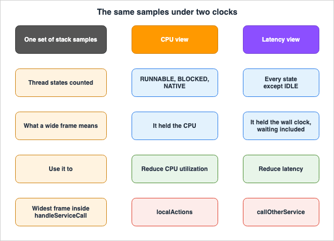

This is the point this article presses hardest:

Do not write that something is heavy without naming the view the thickness came from. A statement without it points half your readers at the wrong optimization target.

The practical implication is this: If you came here to bring p99 latency down, the default CPU view is not aimed at your goal. The CPU view is a picture for reducing CPU utilization, and it does not show waiting. Optimizing the thickest frame in the default view during a latency investigation means that, where waiting dominates, you optimize a place that is not spending the time.

Conversely, if you came to reduce instance size by cutting CPU usage, looking at the Latency view might lead you to misidentify frames that have become thick due to waiting as being CPU-intensive.

⚠ One important note: In the initial release of Python, the CPU view and Latency view were not supported. The user guide states:

The CPU view and latency view were not supported for first release of Python applications; if you
open old Python profiles from before February 2021, the profiling data represents wall clock time
percentages for each frame.

When opening older Python profiles, you will always be viewing data based on wall clock time, regardless of the view you select.

4. Reading the Graph Without Over-Reading It

4.1 Three Visualizations

CodeGuru Profiler offers three visualizations, each providing a different perspective on the same profile.

Visualization	Direction	Use Case
Overview	Bottom-up. The bottom holds the entry points, and as you move upward, you delve deeper into the call stack.	Trace the call paths to identify the routes leading to inefficient code.
Hotspots	Top-down. The functions consuming the most time sit at the top.	Identify functions themselves that have a high computational cost.
Inspect	Focuses on a single frame, specified by name.	Collect instances of a frame that appear in numerous locations and view them in one place.

⚠ The Overview visualization can make it difficult to identify issues that are spread across multiple call stacks. The user guide provides the example of logging calls, suggesting that in such cases, the Hotspots view is more suitable. This choice is not about how to interpret the data; if you are looking for issues that are distributed, no matter which view you choose, the Overview will not effectively highlight them.

4.2 What the User Guide Says the Graph Does Not Tell You

It is valuable to retain the limitations that the user guide itself explicitly lists. Three things do not come off the overview.

First, the order of calls cannot be read.

Inside main code, the doOne function is called before the doPlenty function. Frames are ordered
alphabetically, and from the visualization, we can't tell in which order the functions are called.

Frames sit in alphabetical order, not call order. Attempting to read them chronologically from left to right is incorrect.

Second, the number of calls cannot be read.

The doOne function is called more often than the random function. The overview visualization only
tells that more CPU time is spent in doOne but CodeGuru Profiler doesn't give any information about
the number of times it was called.

Third is the It's not a duration. quoted in Section 3.1.

These three points each refute assumptions that users might naturally form when examining the flame graph. "A wider frame means it is slower." "A frame on the left means it was called first." "A thicker frame means it was called more frequently." None of these assumptions hold true.

4.3 What an Idle Application Looks Like

There is one more typical way to misread the picture. It is the state where almost no samples were collected in the first place.

Applications with few requests spend most of their time in an idle state. Even when samples are collected, there are very few moments when the code is actually being processed. AWS's blog outlines how to identify this state, and includes the following indicators:

Very small frames are absent. Because there are so few samples, the width of a single sample is wider than usual.
Even in larger frames, the time spent in RUNNABLE or NATIVE states is minimal.
The frame representing the profiler's own overhead, ProfilingCommand.run, is often larger than expected.

The third point is particularly insightful. The profiler's own overhead is visible in the flame graph. When an application is doing very little, the most prominent processing activity often becomes the profiler itself. Attempting to identify optimization targets based on this type of flame graph is ultimately unproductive.

5. Taking the Profile on AWS

⚠ Check the service lifecycle status first. Several services carry the CodeGuru name, and two of them have already been retired. Amazon CodeGuru Profiler is currently available as of September 7, 2026. As of the date of this review, there is no mention of the service lifecycle in the introductory chapter of the user guide or in the document history, and it does not appear on any of the AWS Service Availability Updates lists for October 2025, March 2026, or June 2026.

Other services in the same family have been retired. Amazon CodeGuru Reviewer ended new customer onboarding and entered a maintenance phase as of November 7, 2025. Amazon CodeGuru Security has progressed even further in its lifecycle.

On November 20, 2025, AWS will discontinue support for Amazon CodeGuru Security. After November 20,
2025, you will no longer be able to access the /codeguru/security console, service resources, or
documentation.

⚠ This announcement is currently only available in the AWS CLI and individual SDK reference documentation. The dedicated end-of-support page has already been removed. When researching the retirement of a service, the pages stating the fact of its retirement are the first to disappear.

These three services are distinct, despite having similar names. The history, and what each status takes away, belong to the existing AWS Retired Services History and Timeline and AWS Service Lifecycle States.

⚠ Service lifecycles are subject to change. The information above reflects the status as of the date of this review and should be verified before making any decisions.

5.1 Supported Languages, and Which Document Says So

⚠ Read across the documents and they look contradictory. They are not. Each one describes a different scope.

The opening chapter of the user guide states the supported languages for the service as a whole.

CodeGuru Profiler currently supports applications written in all Java virtual machine (JVM) languages
and runtimes and Python 3.6 or later.

The supported languages include all JVM-based languages and Python 3.6 and later. A feature-by-feature table on the same page confines the language difference to a single row.

Feature	Java / JVM	Python
CPU Profiling	Yes	Yes
AWS Lambda and other AWS compute platforms	Yes	Yes
Anomaly Detection and Recommendation Reports	Yes	Yes
Thread State Color Coding	Yes	Yes
Heap Summary Visualization	Yes	No

The only difference is in the last row. Heap summary visualization runs on JVM languages only. Every other feature covers both.

⚠ The statement "all languages" is not a claim that can be verified through a simple list. The user guide provides code examples for seven languages, under the headings that describe enabling the agent with code.

Java
Scala
Kotlin
Groovy
Jython
JRuby
Clojure

⇒ Those seven are the languages with code examples. They are not the ceiling on supported languages. The opening chapter says all JVM languages and runtimes, which is broader than the list.

⚠ An AWS blog post mentions only Java, Kotlin, and Scala as JVM-based languages, but this post is from 2020. The definitive source for supported languages is the user guide, while the blog post represents a snapshot in time. The same blog post also states that many of the recommendations are tailored for Java, indicating that support and providing recommendations of the same quality are separate considerations.

5.2 One Agent, Several Ways to Attach It

The FAQ states where the agent runs.

Amazon CodeGuru Profiler works with applications hosted on Amazon EC2, containerized applications
running on Amazon ECS and Amazon EKS, as well as serverless applications running on AWS Fargate and
AWS Lambda. Furthermore, you can run Amazon CodeGuru Profiler on-premises.

The way you attach it is decided not by the platform but by the language, and by whether you can touch the code. For JVM-based systems, the user guide provides a table comparing two different paths. Since the same functionality is available through either approach, the choice is not based on features.

Aspect	Command Line (`-javaagent`)	Code
Profiling existing applications	Yes	No (requires recompilation)
Using a custom authentication provider	No	Yes
Controlling the start time of profiling	No (starts at startup)	Yes

⇒ Attach it to an existing application from the command line. Choose the code path when you need to control when profiling starts, or when you need a custom authentication provider. The user guide explicitly states that you can change paths later. Profiling data is stored on the service side, so changing the agent's deployment method will not result in data loss.

Lambda offers a third approach, letting you enable profiling from the function's configuration.

⚠ However, the descriptions of supported runtimes are split across separate pages, one for JVM and one for Python. Reading only one can lead to a misunderstanding of the supported scope.

The JVM page narrows the configuration-only path to specific runtimes.

To start CodeGuru Profiler in your application running on AWS Lambda, you can either update your
Lambda function configuration or modify your application code. The former option is available only
for Java 8 on Amazon Linux 2 and Java 11 and Java 17 (Corretto) runtimes, while the latter is
available for all Java runtimes.

The Python page describes a different scope.

CodeGuru Profiler integration for AWS Lambda is currently available for applications that run on
Python 3.7 up to Python 3.9.

⇒ These two are not contradictory. Each describes its respective language, and attempting to combine them into a single table would inevitably lead to errors. Both pages indicate that the supported runtimes are subject to change.

Lambda carries one more constraint of its own.

You can profile your Lambda functions running in Java if they are called often enough for CodeGuru
Profiler to gather enough samples.

Functions that are called infrequently may not be profiled because sufficient samples are not collected. For functions that complete in under 5 minutes, multiple executions may be necessary. This is a preview of the topic discussed in Section 9, and relates to the very nature of sampling techniques.

5.3 What You Can Tune, and What It Costs You

The service returns settings that adjust the agent's behavior. The AgentConfiguration parameters, as detailed in the API reference, consist of five options.

Valid Keys: SamplingIntervalInMilliseconds | ReportingIntervalInMilliseconds |
MinimumTimeForReportingInMilliseconds | MemoryUsageLimitPercent | MaxStackDepth

Two of these parameters are directly relevant to the subject of this article.

SamplingIntervalInMilliseconds defines the sampling interval. Reducing this value increases the number of samples, resulting in more detailed estimations, but also increases the agent's load. Conversely, increasing the value has the opposite effect. This value directly determines the size of the blind spots, as described in Section 9.1.

MaxStackDepth sets the maximum stack depth. The API reference provides examples illustrating its effect.

MaxStackDepth - The maximum depth of the stacks in the code that is represented in the profile. For
example, if CodeGuru Profiler finds a method A, which calls method B, which calls method C, which
calls method D, then the depth is 4. If the maxDepth is set to 2, then the profiler evaluates A and B.

⚠ If the depth is restricted, data from beyond that point will no longer be present in the profile. In applications with a deep framework layer, setting a low maximum depth can result in the agent being cut off before it reaches your own code, leaving a flame graph that shows only the framework's entry point. The visualization will appear normal, and nothing will seem to be missing.

The service dictates the frequency of transmissions.

How long a profiling agent should send profiling data using ConfigureAgent. For example, if this is
set to 300, the profiling agent calls ConfigureAgent every 5 minutes to submit the profiled data
collected during that period.

The console's summary page states the agent's own load.

The Agent CPU usage provides an estimate of how much of the system CPU resources are consumed by the
CodeGuru Profiler agent on average across profiled instances. It's expected that this value is low
(<1%); however, it can be normal for this to be higher depending on the application being profiled.

⚠ This is the value AWS expects, and not necessarily the actual values observed in your environment. The documentation acknowledges that, depending on the application, actual values may sometimes exceed these expectations. It is more accurate to observe the actual values displayed in the console.

5.4 How Long the Profiles Live

Retention falls into three stages. According to the user guide:

Data received from an agent is aggregated into profiles representing five-minute periods. These are
then aggregated into hourly and daily profiles. CodeGuru Profiler currently retains five-minute,
hourly, and daily profiles for 15 days, 60 days, and three years, respectively.

⚠ Regarding this value, other documents stating a 14-day retention period still appear in search results. The current status of those documents will be addressed in Section 11.1.

The three stages of aggregation have practical implications. A 5-minute profile provides a small sample size and fine-grained detail, but the estimates are less precise. Conversely, 1-hour or 1-day profiles are statistically more stable. AWS blogs also state that, in many cases, a 1-hour or 1-day period provides a more accurate profile.

⇒ To capture the moment of an incident, use a 5-minute profile. To identify trends, use a period of 1 hour or longer. Furthermore, because 5-minute profiles are deleted after 15 days, if you postpone incident analysis, you risk losing the most granular evidence first.

6. Runtime Metrics Are Not Profiles

6.1 What Application Signals Collects

CloudWatch Application Signals collects runtime metrics. Examining only the names and contents of these metrics, it can look as though they overlap with profiling.

Runtime metrics track application metrics over time, including memory usage, CPU usage, and garbage
collection.

The specific items actually collected are quite detailed. For Java applications, Application Signals sends 16 JVM metrics to the ApplicationSignals namespace, carrying the Service and Environment dimensions.

Category	Metric Name
GC Time	`JVMGCDuration` / `JVMGCOldGenDuration` / `JVMGCYoungGenDuration`
GC Count	`JVMGCCount` / `JVMGCOldGenCount` / `JVMGCYoungGenCount`
Memory	`JVMMemoryHeapUsed` / `JVMMemoryUsedAfterLastGC` / `JVMMemoryOldGenUsed` / `JVMMemorySurvivorSpaceUsed` / `JVMMemoryEdenSpaceUsed` / `JVMMemoryNonHeapUsed`
Threads and Classes	`JVMThreadCount` / `JVMClassLoaded`
CPU	`JVMCpuTime` / `JVMCpuRecentUtilization`

For Python applications, it collects 9 metrics. These include PythonProcessGCCount, generational counts from PythonProcessGCGen0Count to PythonProcessGCGen2Count, PythonProcessVMSMemoryUsed, PythonProcessRSSMemoryUsed, PythonProcessThreadCount, PythonProcessCpuTime, and PythonProcessCpuUtilization.

⚠ JVMGCOldGenDuration and JVMGCYoungGenDuration, along with their corresponding Count metrics, are only available in G1. The user guide specifies that they are Available only in G1. If you change the GC algorithm, these four metrics will silently disappear.

6.2 Where the Boundary Falls

This is the point of the chapter.

Runtime metrics provide aggregated values, not a stack trace.

JVMGCDuration tells you the total time spent on garbage collection. It does not tell you which objects triggered the garbage collection. JVMCpuRecentUtilization reports CPU utilization. It does not tell you which functions consumed the CPU. JVMThreadCount reports the number of threads. It does not tell you where those threads are blocked.

Question	Runtime Metrics	Continuous Profiling
Is CPU utilization increasing?	Yes (as a time-series metric)	The summary page shows the average over the last 12 hours, but it is not a tool for tracking it over time.
How much time was spent on garbage collection?	Yes	No
Is the heap continuously growing?	Yes	The heap summary answers this. But it is JVM-only, off by default, and, as Section 7.1 sets out, not recommended in production.
Which functions consumed the CPU?	No	Yes
Which call is waiting?	No	Yes (via the Latency view)
Is a notification needed when a threshold is breached?	An alarm can be set.	Anomaly detection is a separate mechanism, and SNS notification can be configured.

⇒ These two are not alternatives. They stand in sequence. Runtime metrics tell you when something happened. Continuous profiling tells you what was running at that moment. With only one of them you either know when something happened but not why, or you can see candidate causes but not when they struck.

⚠ It is incorrect to assume that if you have runtime metrics, you do not need continuous profiling. Metrics are the result of aggregation, and aggregation inherently involves discarding details.

6.3 The Language Coverage Does Not Match the Service's Own

⚠ This is easy to read wrong, and the two readings sit on the same page.

The Application Signals core service supports four languages.

Application Signals supports Java, Python, Node.js, and .NET applications.

But runtime metrics do not cover all four. The user guide explicitly states this.

Runtime metrics are not collected for Node.js applications.

⇒ Node.js services will appear in Application Signals, but only the rows related to runtime metrics will be empty. They will also appear in the service map and SLOs. Only the memory and GC time series data are missing.

Runtime metrics also carry prerequisites. The CloudWatch agent must be 1.300049.1 or later. If the Amazon CloudWatch Observability EKS add-on is in use, it must be 2.30-eksbuild.1 or later. Each language then has its own minimum version of the AWS Distro for OpenTelemetry SDK: 1.32.5 or later for Java, 0.7.0 or later for Python, and 1.6.0 or later for .NET.

⚠ The description of supported languages is inconsistent between the introduction and the main body of this page. This is covered in Section 11.

7. What the Heap Summary Adds

Following the CPU and wait time, memory is next, and this is one area where differences still persist across programming languages. The only row in the Section 5.1 table where Python is marked No is the heap summary.

7.1 It Is Off by Default, and Not Recommended in Production

⛔ This section contains the most critical point to understand. Heap summaries operate under a different premise than the always-on functionality discussed in previous sections.

First, nothing is gathered until you turn it on. The user guide uses the term opt in. There are three ways to enable them, corresponding to the agent's deployment method.

Deployment Method	Enablement
Command Line (`-javaagent`)	Add the argument `heapSummaryEnabled:true`.
Code	Call `.withHeapSummary(true)`.
Environment Variable	Set `AWS_CODEGURU_PROFILER_HEAP_SUMMARY_ENABLED` to `true`.

Second, and this is important: the user guide does not recommend enabling heap summaries in production environments.

It is not recommended to enable heap summary data collection in your production environments, as it
might increase latency in your application.

⇒ The claim of low overhead, mentioned in Section 2.1, refers to CPU profiling. Heap summaries are separate, and AWS does not recommend enabling them in production. Do not extend the concept of always-on functionality suitable for production to include heap summaries.

⚠ This note sits on the agent configuration page, not on the page that describes what the heap summary shows. A reader who is only looking into how the heap summary reads can enable it without ever meeting this sentence.

There are also two prerequisites. The Java agent must be version 1.2.6 or later, and the JDK must be OpenJDK8u262b01 or later, or any version of OpenJDK11. The troubleshooting page notes that if the JDK is not supported, a log message indicating that JDK Flight Recorder is unavailable will appear, and it gathers no data.

7.2 What You See Once It Is On

The Heap Summary displays two lines and one table.

Total Capacity is the maximum heap size configured in the JVM, as the user guide states: This value is equal to your JVM's Xmx value (if configured).

Used space is the room the objects surviving a garbage collection cycle need. The user guide provides two ways to interpret this value.

If this value continuously grows over time until it reaches total capacity, then that could be an
indication of a memory leak.

The table contains a threshold; failing to consider it can lead to incorrect conclusions.

Only object types that consume more than 0.5% (by default) of your heap's total capacity across all
objects are detected. Object types with consumption below that threshold are counted as part of the
used capacity value, and are not shown individually in the table.

⇒ The table omits any type below 0.5%. Their bytes still count toward the used space figure. The sum of the sizes of the types listed in the table will not reach the Used space value. This is by design, not a deficiency.

Types that cross the threshold carry a marker. Any type that dropped below the threshold at some point carries an Incomplete data badge, and the value shown averages only the data that was captured. The average leaves out the stretches where that type sat below the threshold.

⚠ The Heap Summary shows a snapshot of objects that the garbage collector was unable to reclaim. The user guide defines Used space as the space required to hold objects on the heap after a garbage collection cycle. A workload that creates many temporary objects and reclaims them quickly leaves no trace here.

The sizes listed for each type in the table represent their "shallow" size, meaning they do not include the size of the objects referenced by that type.

8. Where AWS-Native Coverage Stops

8.1 The OpenTelemetry Profiling Signal

Continuous profiling is an area increasingly being standardized as the fourth signal of observability, and its current maturity is stated explicitly, in a form worth tracking.

OpenTelemetry's conceptual documentation defines "profile" as follows:

A profile is a collection of samples and associated metadata that shows where applications consume
resources during execution.

And the same page states its status explicitly:

Status: Alpha

This Alpha status was announced in March 2026. The OpenTelemetry blog states that profiles have entered public Alpha, allowing the community to use them widely and provide feedback.

⚠ However, within OpenTelemetry, there is not a single label to represent this state. The OTLP specification 1.11.0 states the following:

Status: Stable for the trace, metric and log signals. Development for the profiles signal.

In separate official documentation from the same organization, different labels such as "Alpha" and "Development" are used. Both agree that it is not stable, so the practical judgment does not change. Profiles are not yet at a stage where they can be treated in the same way as traces, metrics, and logs. This is covered in Section 11.

The direction, however, is more concrete. OTLP profiles start from the pprof format, and data converts between the two without loss. Furthermore, profiles can include trace IDs and span IDs, allowing stack samples taken within a specific span to be linked back to that span. If that lands, the place where the trace stops in Section 1 gets closed on the signal side.

⚠ However, it is currently in Alpha. It is not yet appropriate to incorporate it into production observability infrastructure. The information in this section is current as of September 7, 2026, and the level of maturity may change. It is necessary to consult the latest official OpenTelemetry documentation when reading this. ⛔ AWS documentation is not the definitive source for this assessment.

How OpenTelemetry is integrated with AWS, and what capabilities are available for traces, metrics, and logs, is the subject of the existing OpenTelemetry-Native Observability on AWS. That article also cites the same passage from the OTLP specification, confirming that the state of profiles being "Development" was already documented as of August 9, 2026. At the time of writing this article, the version remains 1.11.0.

8.2 Language and Open Source Profilers

Two separate situations sit behind this.

First, there are languages that CodeGuru Profiler does not support. As mentioned in Section 5.1, its support is limited to JVM-based languages and Python. Go, Node.js, Rust, and .NET are not included. If you need to profile production stacks in these languages, your options are either a language-specific profiler or an open-source profiler that you manage yourself.

Second, even for languages that are supported, there may be situations where more granular control is required. Requests for shorter sampling intervals or profiling of allocations and locks, for example, fall outside the scope of the managed service's capabilities. In these cases, it is not that the language is unsupported; rather, you are seeking to collect different types of data.

The existing Incident Triage Flowcharts document lists tools for different languages, mentioning pprof for Go, py-spy for Python, and async-profiler for JVM. Note that the latter two are for languages CodeGuru Profiler already supports. These are presented as options, not replacements.

AWS itself also provides articles outlining alternative approaches. The AWS Containers blog, for example, details how to apply async-profiler to a Java application running on Amazon EKS, using it for both on-demand and continuous profiling, and storing the results in Amazon S3.

⚠ This demonstrates that a process exists, but it does not represent an AWS recommendation. If you choose to manage the profiler yourself, you will be responsible for designing your own solutions for data storage, retention, visualization, and access control. That is the part the managed service was carrying.

8.3 Three Areas This Article Does Not Cover

Some areas look adjacent but have a different subject and different tools. They are named here.

Profiling on Accelerators. Determining how time is spent on devices like Trainium and Inferentia belongs to the Neuron toolset, and to the existing Programming AWS Trainium with the Neuron Kernel Interface.
The Mechanics of eBPF. While eBPF-based profilers exist, understanding what eBPF loads onto a node and where it performs observations is covered by the existing eBPF on Amazon EKS.
Workload Generation. You collect profiles while a workload is running, but generating that workload belongs to the existing Load Testing on AWS.

9. What Sampling Never Tells You

Even with continuous profiling, there are aspects that simply will not be reflected in the data. This is not due to limitations in implementation, but rather a characteristic of the sampling method itself.

9.1 Work Shorter Than the Sampling Interval

By default, the agent samples the stack once per second. If a process is not actively running at that precise moment, it effectively ceases to exist as far as the profiling is concerned.

Suppose a function completes in 50 milliseconds and is called once per second. The probability of it being captured in a sample is 1 in 20. While it will likely appear with sufficient profiling duration, a five-minute profile holds only 300 samples, and about 15 of them carry that function.

⇒ Consequently, shorter-running processes appear less impactful in the profile than they actually are. Furthermore, as described in Section 4.2, the number of calls is not displayed, so it is impossible to determine from the flame graph whether a process appears less impactful because it genuinely consumes fewer resources or simply because it was not captured in any samples.

Reducing the SamplingIntervalInMilliseconds can mitigate this blind spot, but it introduces a trade-off with the agent's overall load.

9.2 Rare Events

Determining the proportion that a frame occupies within a profile is not about how frequently it occurs, but rather the proportion it occupies on the timeline. This is an area where intuition can easily mislead, so it is important to use numbers to verify.

Suppose a process takes 10 seconds and runs once an hour. Within a one-hour profile, this process is running for 10 seconds, which is 10 out of 3,600 seconds, or roughly 0.28% of the elapsed time. If the sampling interval is the default one second, this process is expected to appear in approximately 10 of the 3,600 samples in a one-hour profile.

⇒ Even if the frequency is the same, processes that take longer to complete will appear wider in the profile. A process that runs once an hour and finishes in 1 second is 1 out of 3,600, one tenth of the width of the 10-second process. Rare occurrences should not be mistaken for insignificant events.

The problem is that 0.28% frames may go unnoticed on the flame graph. There are several other frames that appear significantly wider. And unlike the 0.5% threshold used with heap summaries (as seen in Section 7), the flame graph has no lower limit, so small frames can remain small and be overlooked.

⚠ The way you select the window can reverse the appearance. If you choose a 5-minute profile, the 10-second process becomes 10 seconds out of 300, representing 3.3%, which appears much wider than it would in a one-hour profile. Conversely, if you select a 5-minute interval where this event did not occur, it will completely disappear.

⇒ When searching for rare and lengthy events, it is better to first identify the time of occurrence and then select a short window, rather than using a long, averaged window. The information about when the event occurred does not come from the profile. It comes from the metrics and traces. CodeGuru Profiler can also detect anomalies based on the profile's trends and, if configured, can send notifications via Amazon SNS. However, even anomaly detection looks at aggregated profiles, so if a sample was not included, it will not appear in anomaly detection either.

9.3 Off-CPU Waiting

Latency view displays wait times, but the wait times it shows are based on certain conditions.

Latency view only counts thread states that are not IDLE, which inherently assumes that a thread exists. If a thread has not been created, or if the thread pool is exhausted and tasks are waiting in a queue, the waiting entity will not appear as a thread state.

⚠ This is not something the user guide states; it follows from the way sampling works. Since samples are taken as thread stacks, wait times that do not involve a thread stack cannot be captured.

The same principle applies to wait times outside of a process. This includes the time a thread was not allocated a CPU by the kernel scheduler, the time a container was limited by its CPU quota, or the time the host system was waiting due to overload. These types of wait times are difficult to express as a thread state inside the application.

⇒ Therefore, the wait times displayed by Latency view represent wait times that the application itself has actively initiated. Time spent waiting due to external factors requires a different tool to observe.

9.4 Call Counts and Durations

As quoted in Section 4.2, this is a limitation the primary source states outright. Flame graphs do not reveal how many times a particular function is called, nor how long each call takes.

⇒ Consequently, flame graphs cannot differentiate between a function that is called infrequently but performs a computationally intensive task, and a function that is called frequently but performs a relatively lightweight operation. Both may appear with the same visual width. Furthermore, the appropriate solutions for addressing these two scenarios are entirely different: optimization is required for the former, while reducing call frequency is the solution for the latter.

⚠ This is an area where distributed tracing can provide answers. Spans contain information about both the number of calls and the duration. Section 1 said the trace stops. The division of labor also runs the other way at the same time. Leaning entirely on either one always blinds you to the other side.

10. Failure Modes and Anti-Patterns

⚠ The following are all instances that do not trigger any mechanical checks. The picture renders, the agent runs, and nothing raises an error.

Issue	What Happens	Avoidance
Investigating latency while using the default view.	The CPU view does not show waiting. Where waiting dominates, you pick a frame that is not spending the time as your optimization target.	Switch to the Latency view when investigating latency. Always specify which view you are using in your descriptions.
Reading frame width as a duration.	A light function called many times is mistaken for a function that is heavy on each call.	Frame width represents a percentage of samples. Capture counts and durations using traces.
Reading frames from left to right in chronological order.	Frames are sorted alphabetically, not in the order they were called. You may misinterpret the call sequence.	The order cannot be determined from the flame graph.
Grouping the entire fleet into a single group.	Anomalies on a specific machine are diluted into the average and become hard to detect.	Divide the groups to focus on areas where anomalies are suspected. However, this will also reduce the sample size.
Setting `MaxStackDepth` too low.	The stack may be truncated before your code is reached. The resulting visualization may appear normal, but crucial information may be missing.	Set the value considering the depth of the framework layers.
⛔ Enabling heap summaries in production.	The user guide does not recommend enabling this in production, as it can increase latency.	The low-overhead claim in Section 2.1 is about CPU profiling. Do not extend it to the heap summary.
The heap summary shows nothing, and the configuration is never suspected.	Heap summaries are not captured by default. Additionally, agent 1.2.6 or later and a compatible JDK are required.	Explicitly enable it through one of the three opt-in paths and verify your JDK version.
Comparing the totals in the heap summary table with the total used space.	Types accounting for less than 0.5% will not appear in the table, so there will always be a discrepancy.	The table lists only the major types; it is not a comprehensive breakdown.
Selecting targets for optimization based on profiles of idle applications.	The profile contains very few samples, and the profiler's own frames may dominate.	First examine the ratio of `RUNNABLE` and `NATIVE` frames.
Assuming profiling is unnecessary because runtime metrics are being collected.	Aggregated metrics do not provide a breakdown. While you can determine when something occurred, you will never know which function was involved.	Keep both, as a sequence rather than a choice.
Waiting for runtime metrics in Node.js.	These are not captured, so the results will never appear.	First confirm the supported scope.
Searching for rare, heavy events using a long-duration profile.	A 10-second process that runs once an hour is only 0.28% of a one-hour profile, and is lost among the wider frames.	Identify the time the event occurred using metrics and traces, and then create a short window profile containing that specific time.
Leaving the incident's profile to be analyzed later.	Profiles with a 5-minute granularity are lost first.	Assume that the finest-grained evidence will disappear first.

11. Where the Primary Sources Disagree

Writing this article surfaced three places where the official AWS and OpenTelemetry documents disagree in ways a reader will hit at the same spot. It also surfaced one case where a cited source was withdrawn during the investigation.

They are recorded here because any reader who follows the same research path will stop at the same places.

⚠ All of these were measured on September 7, 2026, and either side can be updated.

11.1 The 14-Day Figure Comes From a Document That Has Been Withdrawn

The CodeGuru Profiler user guide states that the retention period for 5-minute granularity profiling data is 15 days.

CodeGuru Profiler currently retains five-minute, hourly, and daily profiles for 15 days, 60 days, and
three years, respectively.

⚠ When searching for this topic, you may encounter materials that state a 14-day retention period. For example, an AWS whitepaper, Security in Amazon CodeGuru Profiler, previously stated a 14-day retention period for 5-minute granularity, 60 days for 1-hour granularity, and 3 years for 1-day granularity.

⛔ However, this whitepaper has already been discontinued. As of September 7, 2026, any page under docs.aws.amazon.com/whitepapers/latest/security-in-codeguru-profiler/ returns a 301 redirect, leading to the entrance page for CodeGuru documentation. The individual pages themselves no longer exist.

⇒ Currently, the only valid source of information indicates a 15-day retention period. The number 14 is simply a remnant of discontinued documentation, persisting in search results and cached data.

⚠ This situation offers a valuable lesson about research methods. Search engine indexing can return content from discontinued pages, presenting it with the same appearance as active pages. This is the same shape as the CodeGuru Security end-of-support page noted in Section 5, which has also been taken down. Therefore, before quoting any information, it is essential to verify that the page still returns a 200 status code, confirming its validity.

11.2 The Language Coverage of Application Signals Runtime Metrics

The CloudWatch user guide's section on runtime metrics lists two languages in its introductory text.

Application Signals uses the AWS Distro for OpenTelemetry SDK to automatically collect
OpenTelemetry-compatible metrics from your Java and Python applications.

However, the same page's prerequisites mention a specific .NET SDK version, and the main body of the page includes a section on .NET runtime metrics, along with tables for DotNetGC-related metrics. Furthermore, the same page explicitly excludes languages that are not supported.

Runtime metrics are not collected for Node.js applications.

⇒ Therefore, the Java and Python languages mentioned in the introductory text have a narrower scope than the content described in the main body of the page. This article takes the main body's perspective and treats Java, Python, and .NET as the three supported languages.

11.3 The Maturity Label of the OpenTelemetry Profiling Signal

As mentioned in Section 8.1, the conceptual documentation states Status: Alpha, while the OTLP specification 1.11.0 indicates Development for the profiles signal.

This is not necessarily a contradiction, but rather a situation where two different documents use different terminology. OpenTelemetry has a system of terms to represent the maturity level of its specifications. "Alpha" refers to a stage where the specification is released for broad use and feedback, while "Development" describes the state of the specification document itself. Neither term indicates the same level of stability as trace, metric, and log data.

11.4 Whether the Heap Summary Belongs in Production

This is not a discrepancy in numbers, but a difference in emphasis. It is recorded anyway, because it changes what a reader decides to do.

The introductory chapter of the user guide lists understanding heap usage as one of the capabilities of CodeGuru Profiler.

Understand your application's heap utilization over time.

The AWS DevOps blog also ties being always on to seeing how memory moves over time, in a single sentence.

Because CodeGuru Profiler is a low-overhead, production profiling service designed to be always on,
it can capture and represent how memory utilization varies over time, providing helpful visual hints
about the object types and the data types that exhibit a growing trend in memory consumption.

However, the page that configures the agent does not recommend enabling it in a production environment.

It is not recommended to enable heap summary data collection in your production environments, as it
might increase latency in your application.

⇒ The documents that introduce the feature discuss the heap summary in an always-on context, while the document that describes the configuration tells you to avoid production. Following the general rule that a sentence written to state a constraint is the more accurate one, this article takes the configuration page.

12. Frequently Asked Questions

Q. Is it safe to keep continuous profiling enabled?

A. That is what AWS designed it for. CodeGuru Profiler is designed to run on production with low overhead. This is AWS's claim, and this article does not present independent measurements. The Agent CPU usage on the console summary page shows the real figure. The user guide states that less than 1% is an expected value, but acknowledges that higher values may also be normal depending on the application.

Q. Which view, CPU view or Latency view, should I use by default?

A. It depends on your goal. If you want to reduce CPU usage or downsize your instance, use the CPU view. If you want to reduce latency, use the Latency view. CodeGuru Profiler defaults to the CPU view, so if you are investigating latency issues, you will need to explicitly switch to the Latency view.

Q. Should I optimize the thickest frame in the flame graph?

A. No. The meaning changes depending on which view you are using. Furthermore, the thickness does not represent either duration or call count. The user guide explicitly states It's not a duration. Thick frames are a starting point for investigation, not a conclusion.

Q. If tracing is already in place, is profiling still needed?

A. Neither replaces the other, and that holds in both directions. Tracing provides information about call counts and durations, and can identify causal relationships across services. Profiling, on the other hand, shows which functions consumed time within a span. Tracing stops at the span boundary, and profiling does not carry call counts or durations.

Q. Are the runtime metrics from Application Signals sufficient on their own?

A. No. Runtime metrics are aggregated values and do not provide a stack trace. They can tell you how many milliseconds were spent on garbage collection, but they will not tell you which objects triggered the garbage collection. The two are not alternatives. They stand in sequence. Metrics tell you when, and the profile tells you what was running then.

Q. Can I see the heap summary in Python as well?

A. No. According to the feature compatibility table in the user guide, only heap summary visualization is marked as No for Python. CPU profiling, support for compute infrastructure including Lambda, anomaly detection and recommendation reports, and thread state color coding are all Yes for Python. The only language-specific difference is this single entry.

Q. Is it acceptable to keep heap summaries enabled constantly?

A. ⛔ No. The user guide does not recommend enabling it in production environments (as it may increase latency). Furthermore, it is not enabled by default and requires explicit opt-in. The always-on discussion running through this article from Section 2 onward is about CPU profiling. The heap summary sits outside it. It is reasonable to enable it temporarily, understanding the potential impact, when there is a need to investigate memory issues.

Q. Can Lambda functions be profiled?

A. Yes, but it depends on how frequently they are invoked. The user guide states that the function has to be called often enough for CodeGuru Profiler to gather enough samples. For functions that complete in under 5 minutes, multiple executions may be necessary. Separate pages carry the supported runtimes for JVM and for Python; reading only one of these pages may lead to an inaccurate understanding of the supported range.

Q. Is it worth waiting for the OpenTelemetry profiling signal?

A. Not as a dependency yet. As of September 7, 2026, the conceptual documentation is in Alpha, and the OTLP specification 1.11.0 lists profiles as being in the Development stage. It is not yet suitable as a foundation for a production-level observability platform. The design aims to include trace IDs and span IDs in the samples, and pprof data is stated to convert to and from OTLP without loss. The level of maturity may change, so it is necessary to consult the official OpenTelemetry documentation at the time of your decision.

Q. What if the language is not supported?

A. Check the supported languages first. CodeGuru Profiler supports JVM-based languages and Python 3.6 and later, so Java, Scala, Kotlin, and Python do not apply to this question. Languages that do apply include Go, Node.js, Rust, and .NET. In these cases, you will need to manage your own profiler for that language. Go, for example, has pprof. However, you will be responsible for designing the storage location, retention period, visualization, and access control. That is the part the managed service was carrying.

13. Summary

Tracing stops at the boundaries of spans. Continuous profiling takes what is running inside those spans, from production, which essentially means periodically inspecting the call stack and counting its contents.

The most important point this article wants to emphasize is that flame graphs have two different "clocks." The CPU view counts RUNNABLE, BLOCKED, and NATIVE states, while the Latency view counts all states except IDLE. These are two different perspectives on the same sample data, and the thickest frames can appear to switch places. Without specifying which view you are looking at, stating that "this is slow" can lead to incorrect conclusions.

Furthermore, the width in a flame graph does not represent duration. The user guide states It's not a duration. The call order and frequency are also not discernible from a flame graph.

Application Signals runtime metrics cannot replace this tool. They tell you about aggregated values, while profiling reveals what was happening at a specific point in time. They are not alternatives. They stand in sequence.

⛔ The ability to run continuously in a production environment is a characteristic specifically of CPU profiling. Heap summaries are not enabled by default, and the user guide does not recommend enabling them in production environments. Of everything in this article, this is the step a reader is most likely to take by mistake.

However, sampling inherently has structural limitations. It misses short-duration processes, rare events, waits that do not appear as thread states, and the relationship between call counts and durations. These are not limitations of the implementation, but inherent characteristics of the technique. Adding more profilers will not fill these gaps. Addressing them requires a different type of observation.

⚠ Availability, supported languages, and signal maturity can move from the verification date of September 7, 2026. The supported runtimes in particular, and the maturity of the OpenTelemetry profiles signal, have to be looked up again before either is used to decide anything.

14. References

References:
Tech Blog with curated related content

Written by Hidekazu Konishi