hidekazu-konishi.com

Disaggregated Prefill and Decode for LLM Serving on AWS - The KV Transfer, the Routing Threshold, and What Disaggregation Does Not Fix

First Published: 2026-08-20
Last Updated: 2026-08-20

If you serve open-weight models yourself, you run into the same wall at some point. You add continuous batching, you add a paged KV cache, and you push concurrency up. What stretches is not the wait for the first token, but the time between tokens after that. Furthermore, this increase is unpredictable. Occasionally, a single, long prompt can halt token generation for unrelated requests.

The cause is known. LLM inference has two phases with different characters, and they sit on the same GPU. The prefill phase processes the entire input prompt in parallel to create the initial KV cache, and its performance is limited by computational speed. The decode phase generates tokens sequentially, relying on memory bandwidth to read both the model weights and the continually expanding KV cache. When these phases share the same GPU, the decode phase is forced to wait while the prefill phase runs for extended periods.

There are two primary approaches to address this. One involves dividing the prefill phase into smaller chunks, interleaving them with the decode phase – a technique exemplified by vLLM's chunked prefill. The other is to disaggregate the phases themselves onto separate GPU pools. This article focuses on the latter approach, which Amazon SageMaker HyperPod offers as Disaggregated Prefill and Decode (DPD). According to the release notes, HyperPod Inference Operator v3.2 shipped on June 12, 2026, and the What's New announcement is dated July 6, 2026. Enabling it simply requires adding a pdSpec to the InferenceEndpointConfig.

This article does not focus on how much faster it becomes. Instead, it explores what you newly have to operate as a result of disaggregating. This is not a matter of modesty, but rather a reflection of how to interpret primary source materials. The official vLLM documentation states the following regarding this feature:

Disaggregated prefill DOES NOT improve throughput.

AWS, meanwhile, publishes benchmark figures showing throughput improving by up to 35 percent and up to 64 percent. Neither claim is inaccurate. The difference lies in what is being measured. Chapter 7 resolves the difference.

Three conclusions are worth stating up front.

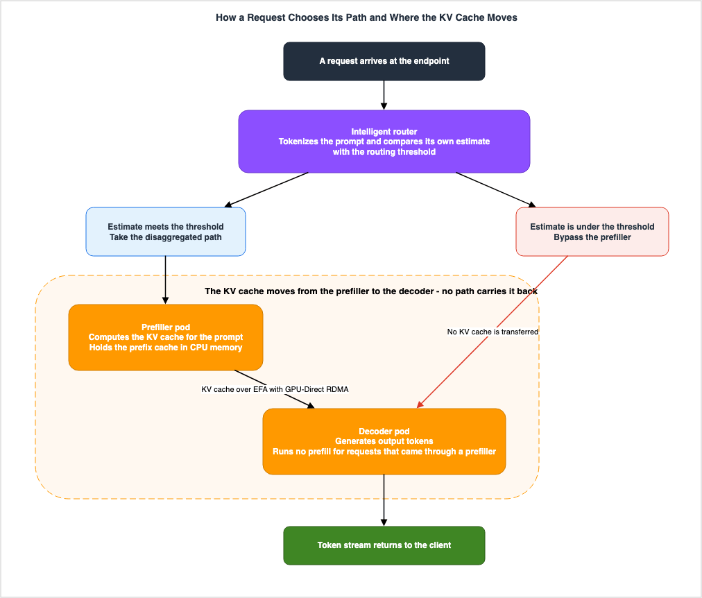
First, requests below the threshold do not pass through the prefiller. The router examines the length of the input and, for requests that fall below the threshold (default: 4,096 tokens), bypasses the prefiller and sends them directly to the decoder. For short prompts, the fixed cost of moving the KV cache outweighs the benefit of isolating decode. Therefore, the understanding that disaggregating makes everything faster is fundamentally at odds with the design principles of this feature.

Second, the capacity that can be increased is on the prefiller side, not the decode side. Whether a request takes the disaggregated path or the direct path, it ultimately reaches the decoder. The decoder is on the critical path for all traffic, while the prefiller is not. Furthermore, the current release explicitly states that it is possible to increase the number of prefillers. This asymmetry is also the point on which the documents disagree most.

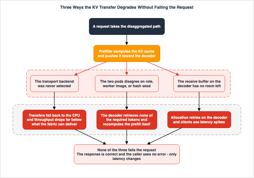
Third, the transfer of the KV cache represents both a new bottleneck and a new failure mode. The transfer can degrade without producing an error. The AWS troubleshooting page states the symptom as a number rather than an exception: transfer throughput below 1 GB/s. A mismatched hash seed alone is enough to stop the transfer from landing, and in that case too the decoder does not crash. It redoes the prefill itself.

Every specification in this article was checked against official documentation. The verification date is August 18, 2026. That verification turned up nine discrepancies between the four AWS documents and the upstream open source documentation, all describing the same feature. Three of these discrepancies are located in areas where users directly interact with the system. These are summarized in Chapter 8, along with a detailed explanation of how to address them.

On the division of topics, this article deals only with what happens after the phases are disaggregated. The basic configuration of the inference engine, continuous batching, paged KV cache, and node autoscaling are covered in Self-Managed LLM Inference on Amazon EKS. The internal workings of EFA, SRD, and placement groups are detailed in Elastic Fabric Adapter and the AWS Network Fabric. This article does not re-explain these topics; it simply describes the connection where the KV transfer is built upon them.

Table of Contents

1. 1. The Assumption That One GPU Runs Both Phases
2. 2. How the Two Phases Differ
3. 3. What You End Up Carrying Once You Disaggregate
4. 4. Conditions Under Which KV Transfers Become Bottlenecks
5. 5. Turning It On in HyperPod
6. 6. Threshold Routing - Deciding Not to Disaggregate
7. 7. Where Disaggregation Does Not Help
8. 8. Where the Primary Sources Diverge
9. 9. Building It Yourself
10. 10. Deciding Whether to Disaggregate
11. 11. Failure Modes and Anti-Patterns
12. 12. Frequently Asked Questions
13. 13. Summary
14. 14. References

1. The Assumption That One GPU Runs Both Phases

1.1 Intended Audience

This article is intended for readers who serve open-weight models in their own cluster and are experiencing increased latency between tokens as they increase concurrency. You have already implemented continuous batching and paged KV caches, and have experimented with adjusting parameters such as --max-num-seqs and --gpu-memory-utilization. However, you are still encountering issues with the increasing tail latency when processing long prompts.

If you have not reached this stage, it is premature to disaggregate the phases. Disaggregation adds components, and every added component becomes something you operate. Chapter 10 sets out the order of the decision, and there too the first branch is whether any options remain within a single pool.

1.2 What Disaggregating the Phases Actually Separates

What DPD separates is neither models nor data. It is the phases of inference. The same model and its weights are present on both the prefiller GPU and the decoder GPU. The only thing that differs is which GPU runs which phase.

Disaggregation is therefore not an operation that shrinks the model, nor one that uses the GPU more efficiently. In exchange for stopping the interference between the phases, it carries state between them. The state being moved is the KV cache, and the pathway for that movement is the network. This single sentence forms the core of this article.

1.3 Three Conclusions, Stated Up Front

Here are those three points again, in more concrete form.

First, the router uses the threshold to decide, on every request, not to disaggregate. The developer guide describes this behavior as follows:

Token length threshold that routes requests to the disaggregated path. Requests that do
not meet this threshold bypass the prefiller and go directly to the decoder.

Short requests do not take the disaggregated path, and that is by design rather than a defect. The AWS blog further explains the reasoning behind this. Below the threshold, the fixed cost of transferring the KV cache over EFA RDMA outweighs the benefits of isolating the decode process.

Second, both the disaggregated path and the direct path end at the decoder. While only requests exceeding the threshold are routed through the prefiller, the decoder processes all requests. In a structure where only one of the two sits on the critical path, the side the documentation says you can add capacity to is the side that does not.

Third, the transfer degrades rather than fails. As detailed in Chapter 4, it degrades silently for three independent reasons: the capacity of the receive buffer, the selection of the transport backend, and the matching of the hash seed. While this degradation manifests in three different ways, none of them result in request failures. From the user's perspective, the issue is not an error, but rather a slowdown.

1.4 What the Existing Articles Already Hold

This section clarifies what this article will not cover.

Topic	Which article holds it
Basic configuration of inference engines, continuous batching, paged KV cache, Karpenter, ALB	Self-Managed LLM Inference on Amazon EKS
EFA functionality, SRD, ENA Express, placement groups, EFA security group rules	Elastic Fabric Adapter and the AWS Network Fabric
Optimizations for the managed inference side, quotas, provisioned throughput, prompt cache	Amazon Bedrock Inference Throughput and Latency Optimization
Retries, backoff, circuit breaking, stream recovery on the calling side	LLM Inference Resilience Patterns on AWS
Configuration of the Amazon EKS control plane, scheduler scoring strategy, reversibility	Amazon EKS Control Plane Configuration

One word on the last of those. DPD runs on a HyperPod cluster with the EKS orchestrator, so the control plane's scheduler determines which node each Pod is placed on. This article describes only the placement DPD requires, a single Availability Zone and EFA-capable nodes, and does not go into scheduler configuration. Information on the scheduler's parameters can be found in the articles listed above.

Finally, this article will not discuss pricing. Given that a configuration requiring at least two nodes is necessary, cost considerations are inevitable. Prices move, so the AWS pricing pages are the authority.

2. How the Two Phases Differ

2.1 The Resource Profile of Each Phase

AWS documentation briefly describes two phases with distinct characteristics.

Prefill is compute-bound. It processes the entire input prompt in parallel to generate the
initial key-value (KV) cache. Decode is memory-bound. It generates one token at a time and
requires substantial memory bandwidth to access model weights and the growing KV cache.

This leads to two design implications.

First, optimizing one phase does not necessarily improve the other. If you want to speed up prefill, you need to increase the number of processing units. If you want to speed up decode, you need to increase memory bandwidth. Even when residing on the same GPU, choosing a configuration that benefits one phase will inevitably impact the performance of the other.

Second, the optimal degree of parallelization varies for each phase. The official vLLM documentation explains one of the advantages of disaggregation as follows.

This gives you the flexibility to assign different parallel strategies (e.g. tp and pp) to
tune TTFT without affecting ITL, or to tune ITL without affecting TTFT.

Tensor parallelism and pipeline parallelism become adjustable per phase. The llm-d project further translates this into more specific recommendations, suggesting that the prefill phase should utilize a lower degree of parallelism with an increased number of replicas, while the decode phase should utilize a higher degree of parallelism with a reduced number of replicas.

2.2 What Happens When They Are Colocated

The AWS developer guide clearly outlines the specifics of the interference.

When prefill and decode run on the same GPU (colocated), a single long-context request can
stall in-flight token streams for other clients, inflating per-token latency under load.

What matters is who is hurt: not that request, but the other clients. It is understandable that someone who submitted a long prompt might experience delays. What is less intuitive is when another user, who sent a short query, experiences their tokens being interrupted mid-process. When using streaming, this interruption directly translates to a degraded user experience.

Therefore, this issue is not visible when looking at average performance metrics. It only becomes apparent when examining the tail of the token latency distribution. This could explain situations where a system operating with acceptable average performance still receives complaints.

2.3 The Mitigation That Already Exists - Chunked Prefill

Before disaggregating the phases, there is another approach that can be employed while still using a single pool: chunked prefill. This involves breaking down the prefill process into smaller segments and inserting them between decode steps. The official vLLM documentation states the relationship between disaggregation and this technique plainly.

Chunked prefill with a proper chunk size also can achieve the same goal, but in practice
it's hard to figure out the correct chunk size value. So disaggregated prefilling is a much
more reliable way to control tail ITL.

Do not lose the part where it says the same goal can be achieved. The reason disaggregation is said to be preferable is not necessarily due to its superior performance, but rather its reproducibility. The grounds for choosing disaggregation are that determining an appropriate chunk size is difficult in practice.

The AWS blog also presents the information in a similar order, stating that disaggregation controls tail latency more reliably than tuning chunked prefill does. Conversely, if you are able to effectively tailor the chunk size to your specific traffic patterns, the case for moving to disaggregation is that much weaker.

2.4 What Disaggregating the Phases Promises

Pulling the preceding together, disaggregation promises three things.

What it promises	How the primary sources word it
Control of the tail of inter-token latency, which vLLM abbreviates to ITL	vLLM writes Controlling tail ITL, AWS writes more predictable latency under mixed traffic
A different parallel strategy per phase	vLLM writes assign different parallel strategies
Independent scaling of capacity per phase	AWS writes lets you scale each phase independently

Only the third carries a condition in the current release. Section 7.6 and Chapter 8 take it up.

Note what is not in this list: throughput. vLLM states explicitly that disaggregation does not improve throughput. Section 7.1 takes up the figures AWS publishes.

3. What You End Up Carrying Once You Disaggregate

3.1 Three Components and Four Transfer Layers

HyperPod's DPD is composed of three components and a single transfer stack.

Component	What it does
Intelligent Router	Tokenizes prompts, compares them against a threshold, and determines the routing path. For the disaggregated path it selects a prefiller, has that prefiller push the KV cache to a decoder, and then forwards the request to the same decoder.
Prefiller Pod	A vLLM worker that utilizes LMCache as a KV connector. It calculates the KV cache for long prompts and pushes it to the decoder layer by layer, ensuring continuous computation and transfer to prevent GPU idle time.
Decoder Pod	A vLLM worker that receives data through LMCache. It allocates GPU memory for receiving data and begins token generation as soon as the transfer is complete. Because requests that came through the disaggregated path need no prefill, even if long requests are received, ongoing token generation will not be disrupted. Requests below the threshold bypass the prefiller, so the decoder itself performs the prefill operation.

The transport stack has four layers, and HyperPod ships them assembled.

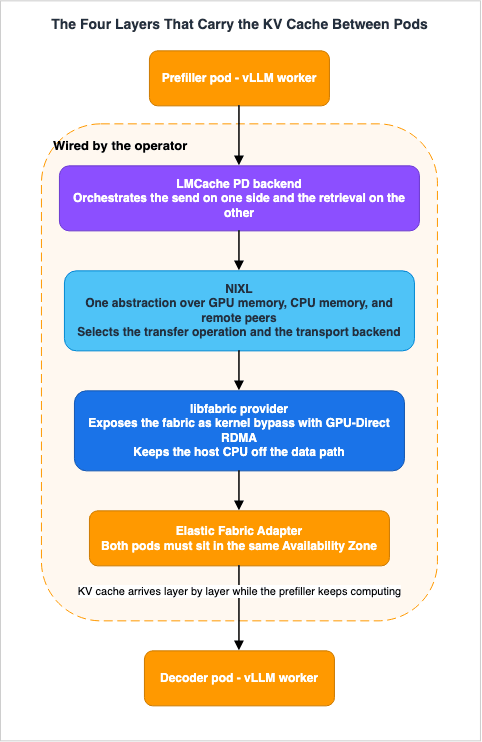
Layer	What it carries
LMCache PD Backend	Manages the transmission from the prefiller side and the reception on the decoder side.
NIXL	Handles GPU memory, CPU memory, and remote destinations using a unified abstraction, selecting the appropriate RDMA operations.
libfabric	Exposes EFA as a kernel-bypass and GPU-Direct RDMA, removing the host CPU from the data path.
EFA	The actual network infrastructure.

AWS states that the transfer cost for these four layers is negligible compared to the prefill calculation cost. On ml.p5.48xlarge, with 3,200 Gbps of EFA, an 8,000-token transfer for Llama 3.3 70B takes single-digit milliseconds. The details of EFA itself are covered in Elastic Fabric Adapter and the AWS Network Fabric, so this article will not delve further into that topic.

3.2 The Transfer Runs in One Direction

As shown in the diagrams and documentation, the KV cache moves in one direction only: from the prefiller to the decoder. There is no reverse path documented.

This asymmetry has two key implications.

First, the prefiller becomes the authoritative source for the prefix cache. The LMCache assigns an L1 cache in CPU memory to each prefiller. When prefixes reappear – such as system prompts, conversation history, or search context – they are supplied from this cache rather than being recomputed on the GPU. AWS describes this as the prefiller being the "source of truth" for cache hits.

Second, KVs generated by the decoder are not saved. The example manifest for HyperPod sets LMCACHE_SAVE_DECODE_CACHE to "False", and AWS explains that this disables redundant L1 caches on the decoder side. The LMCache documentation provides a more definitive explanation of this setting, which will be discussed in Chapter 8.

3.3 Items That Must Be Consistent on Both Sides

From the moment the phases are disaggregated, the prefiller and the decoder become a pair, operating under the assumption that their configurations are aligned. The vLLM NixlConnector compatibility documentation states that a compatibility hash is checked during the handshake, and lists what must agree.

vLLM version and NIXL connector version
Model (architecture, dtype, number of KV heads, head size, number of hidden layers)
Attention backend
KV cache dtype (cache_dtype)
EAGLE/MTP-style speculative method and draft-model configuration
NIXL transfer mode (push vs pull) - a push (WRITE) connector and a pull (READ) connector
use incompatible transfer protocols and must never be paired

This list has operational significance. Actions such as updating only one side's image, changing quantization settings on only one side, or switching the attention backend on only one side, will directly lead to handshake failures. While a single pool allows updating only one replica with a new image – a standard canary deployment – in a disaggregated configuration a canary that crosses the phase boundary does not mean the same thing.

The AWS DPD troubleshooting page also lists, among the checks for a failed KV transfer, that both pods use the same worker image. Knowing the compatibility hash mentioned above provides context for what this check is protecting.

Conversely, the document also explicitly lists items that may differ between the two sides. These include tensor parallelism degree, block size, the number of blocks in the KV cache, and the depth of speculative decoding. However, these items are subject to additional constraints, which are discussed in Section 9.2.

One important note: This description of the compatibility hash specifically applies when using the vLLM NixlConnector directly. HyperPod's DPD utilizes an LMCache PD backend running on top of NIXL, so the same list may not be directly applicable. AWS does not address this point. While the operational conclusion remains that both sides' images should be aligned, it is advisable not to assume that every individual item must be identical.

4. Conditions Under Which KV Transfers Become Bottlenecks

This chapter will address three independent factors that can lead to KV transfers becoming bottlenecks: the capacity of the receive buffer (Section 4.1), the selection of the transport backend (Section 4.2), and hash seed matching (Section 4.4). Section 4.3 will discuss how these factors manifest in logs and metrics. A common characteristic of all three is that they do not cause requests to fail. Instead, the symptoms appear as latency rather than errors, and the specific manifestation of this latency varies depending on the underlying cause.

4.1 Buffers Allocated on the Receiving Side

The decoder pre-allocates a GPU buffer to receive the KV cache. In HyperPod, this is specified by PD_BUFFER_SIZE, with a default value of 8 GiB. That value is per rank.

AWS provides specific details regarding the rationale for the default value. When running Llama 70B with tensor parallelism of 8, the KV cache per token is approximately 40 KB per rank. A 6,000-token prompt would therefore consume approximately 0.23 GB per rank, allowing the 8 GiB buffer to handle roughly 35 such transfers concurrently.

The text also describes the symptoms when the buffer is insufficient.

Failed to allocate memory object, retrying...

When this log appears on the decoder, it manifests as latency spikes on the client side. Possible solutions include increasing the buffer size to 16 GiB or 32 GiB, or increasing the number of decoders. However, AWS notes that increasing the buffer size consumes more GPU memory, and it may be necessary to reduce the --gpu-memory-utilization setting on the decoder.

This behavior was not present in a single-pool configuration. In a single pool, two things divide GPU memory: the weights and the KV cache. Disaggregate, and a third consumer appears on the decoder side, and its consumption increases proportionally to the degree of concurrency.

4.2 The Transport Backend You Have to Select on Purpose

NIXL is an abstraction layer that carries several transport backends. The official vLLM documentation clearly states the default option.

NixlConnector can use different NIXL transport backends (plugins). By default, NixlConnector
uses UCX as the transport backend.

If you want to use EFA, you must explicitly specify a different backend.

vllm serve <MODEL> \
  --kv-transfer-config '{
    "kv_connector":"NixlConnector",
    "kv_role":"kv_producer",
    "kv_connector_extra_config":{"backends":["LIBFABRIC"]}
  }'

Even the reference architecture that AWS publishes for llm-d explicitly mentions LIBFABRIC.

- "--kv-transfer-config"
- '{"kv_connector":"NixlConnector", "kv_role":"kv_both","kv_connector_extra_config": {"backends": ["LIBFABRIC"]}}'

Copy the quoting exactly as it stands. The outer layer should be single quotes, and the inner JSON should be double quotes. Get it wrong when passing it through a shell and the flag is still accepted. Only the setting changes.

NIXL's documentation states that the libfabric plugin requires libfabric version 1.21.0 or later, that GPU Direct RDMA support is required, and that AWS EFA is the network hardware it lists as validated. On EFA-enabled AWS instances it recommends installing libfabric through the AWS EFA installer. That this floor can be higher than the one inherited from an older HPC image, and the library versions as AWS documents them, are covered in Elastic Fabric Adapter and the AWS Network Fabric.

When using DPD with HyperPod, the operator is responsible for configuring this layer. AWS states that if you select a DPD-compatible worker image, the connector, NIXL, and EFA will be automatically connected to all pods. If you build your own setup, this becomes your responsibility. This is covered in Chapter 9.

4.3 Symptoms Appear as Numbers, Not Errors

What happens when a transfer does not reach EFA? The AWS troubleshooting page describes that state with a threshold rather than an exception.

KV transfer throughput below 1 GB/s. EFA is not being used and transfers are falling back
to CPU.

The significance of this line lies in what it does not say. There are no exception names or HTTP status codes mentioned. The request succeeds, and a token is returned. It is just slow. In configurations that only monitor availability and error rates, this degradation will go completely unnoticed.

On the same page, another instance of silent failure is described.

Decoder logs show Retrieved 0 out of N required tokens. KV transfer did not occur and the
decoder fell back to local recomputation.

When a transfer fails to complete, the decoder does not fail the request; instead, it recalculates the prefill on its own. The disaggregated configuration quietly falls back to single-pool behavior. Furthermore, in this state, it operates with twice the GPU usage, but delivers performance equal to or worse than what you had before disaggregating.

The decoder's logs show the healthy state. The normal output shown by AWS takes the following form:

[Worker_TP5] [LMCache INFO] [req_id=cmpl-...] Retrieved 6035 out of 6035 required tokens (from 6035 total tokens).
   size: 0.2344 gb, cost 1.3304 ms, throughput: 176.1686 GB/s

The fact that the required number of tokens matches the number of tokens successfully retrieved, and that the final throughput value significantly exceeds the 1 GB/s threshold mentioned earlier, provides evidence that the transfer is reaching EFA. These two metrics are worth monitoring.

4.4 The Hash Seed Has to Agree or the Transfer Never Lands

A surprising third factor can lead to failures. The HyperPod manifest example sets the following environment variable:

- name: PYTHONHASHSEED
  value: "0"

AWS explains why. LMCache uses Python's built-in hash() function to calculate cache keys for prompt tokens. Because Python randomizes this hash seed by default for each process, even with the same prompt, different keys can be generated between the prefiller and decoder, leading to mismatches and failed lookups. Fixing the seed ensures that keys are consistent across pods.

LMCache's documentation also describes this issue, albeit in more general terms.

For correct KV cache transfer, ensure all processes use the same PYTHONHASHSEED to keep the
hash of the KV cache consistent across processes

What makes this one awkward is three causes and one symptom. When keys do not match, the system reports Retrieved 0 out of N, and the decoder will attempt to re-run the prefill process independently. The AWS troubleshooting page lists three checks for that one symptom: that pd_role is correctly configured (the prefiller should be a sender, and the decoder a receiver), that both pods are using the same worker image, and that PYTHONHASHSEED is set to "0" on both pods. Therefore, simply seeing Retrieved 0 out of N does not tell you which of these three potential causes is at play.

This is a different symptom from the transport backend problem in Section 4.2. When the backend is not using EFA, the transfer itself will still occur, resulting in a consistent number of tokens retrieved. However, the throughput will decrease. Observing the number of tokens retrieved and monitoring the transfer throughput are distinct observations used to differentiate between two separate failure modes.

4.5 Estimating Transfer Costs

The model, the context length, and the degree of parallelism determine the transfer volume. The values provided by AWS refer to running Llama 70B with tensor parallelism of 8, resulting in approximately 40 KB per rank per token. This figure is specific to the configuration and should not be directly applied to different models or parallelism settings.

There are two practical implications for this estimate.

First, the sizing of the buffer is directly linked to the design of the concurrency level. AWS's statement that 8 GiB holds roughly 35 in-flight transfers of about 6,000 tokens each is, read directly, a statement about the ceiling on concurrency. If you plan to increase concurrency, you will need to either increase the buffer size or expand the capacity on the decoder side.

Second, the design of the threshold also influences the overall transfer volume. Lowering the threshold will increase the number of requests that take the disaggregated path, thereby increasing the total transfer volume. Conversely, raising the threshold will decrease it. This will be discussed further in Chapter 6.

5. Turning It On in HyperPod

5.1 Adding a pdSpec

You enable DPD by adding a pdSpec section to an existing InferenceEndpointConfig. The developer guide clearly explains the placement of this field.

Presence of this field is what makes the endpoint disaggregated: the operator creates
separate Deployments for prefill and decode and wires them together via the router and
LMCache PD backend.

The presence of the field, rather than its value, determines the switch. That is also the explanation of how to go back. The developer guide describes the return to a standard colocated deployment as applying a new InferenceEndpointConfig that contains no pdSpec.

The minimal form is as follows:

pdSpec:
  prefillSpec:
    replicas: 1
    resources:
      limits:
        nvidia.com/gpu: ${GPUS_PER_NODE}
      requests:
        nvidia.com/gpu: ${GPUS_PER_NODE}
    args:
      - "--gpu-memory-utilization"
      - "0.75"
  decodingSpec:
    replicas: 1
    resources:
      limits:
        nvidia.com/gpu: ${GPUS_PER_NODE}
      requests:
        nvidia.com/gpu: ${GPUS_PER_NODE}
  routingThreshold: 4096

The fields mean this.

Field	What it means
replicas	The number of prefill and decode instances. The developer guide explains that these can be scaled independently. Refer to sections 7.6 and 8 for details on the extent of this independence.
resources	Applies to that role's pod spec. The DPD pods ignore the top-level worker.resources, and the per-role values win.
routingThreshold	The input token length threshold for sending a request down the disaggregated path.
args	vLLM flags passed only to that specific role. The operator merges them into worker.args at startup, replacing flags that are already there and appending flags that are not.

The handling of resources can be a potential pitfall, especially when compared to the complete example on the same page. The complete example in the developer guide specifies CPU, memory, and GPU under worker.resources, and specifies only GPU under the role-specific resources in pdSpec. However, the same page states that, for DPD pods, the top-level worker.resources is ignored, and role-specific values take precedence. If a user simply copies the complete example into their DPD pod configuration, they may inadvertently lose their CPU and memory specifications.

AWS does not explicitly address this point. It is unclear whether the entire resources section is ignored, or only the keys given per role. While this article does not include empirical validation, as a best practice, it is recommended to write the CPU and memory you need into the role-specific resources as well. The same applies when migrating from a colocated deployment by adding a pdSpec. Verify that any previously effective specifications remain as intended after applying the configuration.

5.2 Prerequisites

DPD relies on several non-negotiable prerequisites.

Prerequisite	What it requires
Orchestrator	Amazon EKS. What's New states HyperPod clusters using the EKS orchestrator explicitly. HyperPod can also be built on Slurm, but DPD is not covered there.
Operator Version	HyperPod Inference Operator v3.2 or later. Earlier versions do not support DPD. A newly created HyperPod EKS cluster carries it by default.
Instances	Must support EFA (Elastic Fabric Adapter) and GPU-Direct RDMA (Section 5.3).
Placement	Nodes must sit in the same Availability Zone. This is a requirement for EFA's high-bandwidth communication.
Worker Image	Must include vLLM, LMCache, NVIDIA NIXL, and the EFA libfabric provider.

Two worker images are on offer as of the verification date.

public.ecr.aws/deep-learning-containers/vllm:server-hyperpod-cuda-v1.1
lmcache/vllm-openai:v0.4.3

The developer guide indicates that both images include LMCache 0.4.3, vLLM 0.19.0, and NIXL 1.0.0. However, these dependencies may change over time, so treat the official page as authoritative for your own build.

The operator version can be verified using the following command:

kubectl get deployment hyperpod-inference-operator-controller-manager \
  -n hyperpod-inference-system \
  -o jsonpath='{.spec.template.spec.containers[?(@.name=="manager")].image}{"\n"}'

The troubleshooting page also describes the symptom of running an operator older than v3.2, such as pods repeatedly restarting due to EngineDeadError or TimeoutError. Identifying an outdated operator version as the root cause of these symptoms can be challenging without prior knowledge. Check the operator version before you start disaggregating.

5.3 Three Ways AWS States Which Instances Work

Three AWS documents describe the same feature at three different strengths. While this discrepancy is also discussed in Chapter 8, this section is included here as it is likely to be encountered first in practical scenarios.

The developer guide writes it as a limit.

Disaggregated Prefill and Decode requires EFA-capable instances with GPU-Direct RDMA support.
The following instance types are supported: ml.p5.48xlarge, ml.p5e.48xlarge, ml.p5en.48xlarge,
ml.p6-b200.48xlarge, ml.p6-b300.48xlarge. Other instance types are not supported for DPD.

The release notes write it as a recommendation.

Recommended instance families: ml.p5.48xlarge, ml.p5e.48xlarge, ml.p5en.48xlarge,
ml.p6-b200.48xlarge, ml.p6-b300.48xlarge.

What's New writes it as a condition.

DPD is available for SageMaker HyperPod clusters using the EKS orchestrator on EFA-capable
instance types in all AWS Regions where Amazon SageMaker HyperPod is available.

And the ML blog adds a note about the families that are excluded.

Although G6, G6e, and G7e instance families do support EFA with RDMA read/write, performance
on multi-GPU instances is bottlenecked by GPU-to-GPU communication over PCIe.

Take the most restrictive description, which is the five instance types in the developer guide. The reasons for this are explained in Chapter 8, but the key point is that a sentence written to state a limit is the most accurate. At the same time, do not drop the blog's supplementary note. It says the G families fail not for want of EFA, but because GPU-to-GPU communication inside the instance runs over PCIe. That is the same limit seen from another side.

For reference, here are the P5-family specifications among the five the developer guide lists, taken from AWS's published values. The verification date is August 18, 2026.

Instance	GPU	GPU memory	Network bandwidth	GPUDirect RDMA
p5.48xlarge	8 x H100	640 GB HBM3	3,200 Gbps EFA	Yes
p5e.48xlarge	8 x H200	1128 GB HBM3e	3,200 Gbps EFA	Yes
p5en.48xlarge	8 x H200	1128 GB HBM3e	3,200 Gbps EFA	Yes

Do not treat this table as an exhaustive list. The set of supported instances can also grow, so check the developer guide's list when you design. The P6-family specifications are left out for the same reason.

5.4 Three Signals to Observe After Deployment

After applying the manifest, the operator creates a prefill Deployment and a decode Deployment in your namespace, and a router Deployment under hyperpod-inference-system.

A normal state looks like this:

NAMESPACE                   NAME                                   READY   STATUS    RESTARTS   AGE
default                     prefill-dpd-test-XXXX                  3/3     Running   0          7m
default                     decode-dpd-test-XXXX                   3/3     Running   0          7m
hyperpod-inference-system   dpd-test-router-XXXX                   2/2     Running   0          7m

The model pods consist of 3 containers (vLLM worker, Nginx reverse proxy, OpenTelemetry collector), while the router pods consist of 2 containers (router, OpenTelemetry collector). Remember those counts. A pod stuck at 2/3 Ready is loading the model. The same page says a cold fetch of Llama 3.3 70B from Amazon S3 takes 5 to 10 minutes.

The second signal is what the developer guide refers to as the most definitive indicator during startup.

Confirm the prefiller reports sender and the decoder reports receiver. This is the single
most discriminating startup signal — if both pods report the same role or neither prints the
line, the operator did not wire DPD correctly.

Verification should look like this:

kubectl logs $PREFILL_POD -n ${NAMESPACE} -c prefill-${DEPLOYMENT_NAME} \
  | grep -oE "'pd_role': '[a-z]+'" | sort -u

kubectl logs $DECODE_POD -n ${NAMESPACE} -c decode-${DEPLOYMENT_NAME} \
  | grep -oE "'pd_role': '[a-z]+'" | sort -u

The expected output is 'pd_role': 'sender' and 'pd_role': 'receiver'. The role names come from LMCache's vocabulary. The LMCache configuration reference defines the valid values for pd_role as "sender" (prefiller) and "receiver" (decoder), and the strings appearing in the logs directly reflect these values.

The third signal is the status of the InferenceEndpointConfig, which, when normal, returns the following string:

DPD prefill and decode deployments are ready

5.5 What You Can Now Observe

When metrics.enabled is set to true, DPD-specific metrics will appear on the HyperPod inference dashboard. However, there is one condition that must be met. The KV cache and intelligent routing pages state that, in addition to setting enabled under the metrics section to true, the value of modelMetrics.port must match the value of containerPort under modelInvocationPort. The DPD page does not mention this condition, so it is a good place to check if the metrics are not appearing.

The developer guide lists eight DPD-specific metrics:

Metric	What it shows
E2E TTFT	Total time to first token, or TTFT, covering prefill, KV transfer, and routing.
Prefill TTFT	Latency of the prefiller alone.
Prefill Queue	Number of requests waiting for prefill.
Decode Queue	Number of requests waiting for the decoder.
Prefill Time	Time spent on prefill calculation.
Decode Latency	Latency per output token, or TPOT.
KV Transfer Time	Time taken to transfer the KV cache from the prefiller to the decoder.
DPD Routing Counts	The count of disaggregated requests versus the under-threshold fallbacks

This list is also a list of what disaggregation added to your operations. In a single pool the things worth watching were the running and waiting request counts, KV cache utilization, TTFT, and tokens per second. After disaggregation the queue splits in two, TTFT splits into two layers, and a new item, transfer time, is added.

The DPD Routing Counts metric is particularly valuable. The share of requests that took the disaggregated path is a direct indicator of whether the threshold settings are appropriate for your traffic. If that share is very low, disaggregation is buying you almost nothing.

6. Threshold Routing - Deciding Not to Disaggregate

6.1 The Decision the Router Owns

The router makes decisions based on its configuration. According to an AWS blog post, it tokenizes the prompt, applies a configurable threshold for the number of tokens, and then determines whether the request takes the disaggregated path or is served end to end on a decoder. For the disaggregated path, the router has the prefiller compute the KV cache and push it to a decoder, then forwards the request to that same decoder.

The router here is not the policy router that sits on the application side. The layer discussed in Self-Managed LLM Inference on Amazon EKS determines, on a per-request basis, whether to process it using its own fleet or to offload it to a managed service. In contrast, the router in this article is the layer that decides the phase route inside the endpoint, and is automatically provisioned by the operator based on the presence of a pdSpec. The two layers can potentially operate on the same request.

The router logs its decision. When the threshold is exceeded, the log entry will read:

[INFO] Conditional routing: estimated_tokens=6750, threshold=4096, disaggregate=True

When the threshold is not exceeded, the log entry will read:

[INFO] Conditional routing: estimated_tokens=12, threshold=4096, disaggregate=False

The default threshold is 4,096. The developer guide provides guidance on adjusting this value, noting that setting it too low can lead to unnecessary KV transfers for short prompts, which degrades TTFT. Setting it too high reduces the number of requests that take the disaggregated path, limiting improvements to TPOT. The guide also states that the default value works well for most workloads.

6.2 The Threshold Applies to an Estimate

Look at those log lines again. The value being compared is estimated_tokens. The threshold meets the router's own estimate, not the model's tokenization.

AWS documentation specifically addresses scenarios where this has practical implications. It provides instructions for a symptom where, despite sending long prompts, not all of them are bypassing the prefiller.

Verify the estimated_tokens value exceeds your routingThreshold. If the token estimate is
lower than expected, the router's tokenizer may be counting differently — try lowering
routingThreshold.

As AWS itself states, the router's tokenizer may be counting tokens differently. Therefore, it is risky to determine the threshold based on the model's context length or the number of tokens counted on the application side. A more reliable approach is to observe the distribution of estimated_tokens as reported in the router's logs, based on actual traffic.

6.3 Every Request Ends at the Decoder

As shown in the diagram at the beginning of this chapter, there are two possible paths, both converging at a single endpoint. Requests exceeding the threshold are routed through the prefiller before reaching the decoder, while requests below the threshold go directly to the decoder.

This structure results in two key observations.

First, the decoder is on the critical path for all traffic. Even if the prefiller fails, traffic below the threshold will continue to flow. However, if the decoder fails, no traffic can be processed. When designing for availability, the weighting applied to the two pods will therefore be different.

Second, the load distribution depends on the distribution of input lengths. With traffic consisting primarily of short prompts, the prefiller will be largely idle, while only the decoder is utilized. Conversely, if the traffic consists mostly of long prompts, both components will be active. With a mix of prompt lengths, the load on the prefiller alone will vary depending on the threshold setting. So the input length distribution, not the GPU count, sets the ratio of prefillers to decoders.

An AWS blog post suggests that for balanced workloads, a 1:1 ratio is a good starting point. However, for workloads that are prefiller-intensive, such as summarization, classification, or retrieval-augmented generation with long contexts, the ratio should be shifted towards the prefiller, such as 2:1 or 3:1. The blog says that if TTFT climbs under load while TPOT stays stable, the prefill side is what is short.

6.4 The Routing Strategy Guidance Splits Between Documents

When multiple prefillers are present, the router needs to choose which one to forward the request to. intelligentRoutingSpec.routingStrategy makes that selection, and it defaults to prefixaware. There are four available strategies:

Strategy	What it does
prefixaware	Sends subsequent requests with the same prompt prefix to the same instance.
kvaware	Sends requests to the instance with the highest KV cache hit rate.
session	Sends requests from the same user session to the same instance.
roundrobin	Distributes requests evenly, regardless of the KV cache status.

Two AWS documentation resources provide conflicting information regarding which prefiller to choose when multiple are available.

The developer guide says this.

For multiple prefill replicas, use roundrobin to distribute load evenly across replicas and
avoid hot-spotting a single prefiller.

That guide's tuning table points the same way, putting roundrobin with multiple replicas and prefixaware or kvaware with a single replica or with shared prefixes.

The ML blog says the opposite.

With multiple prefillers, set intelligentRoutingSpec.routingStrategy on your workload. Use
kvaware for workloads with repeated prefixes (this maximizes L1 cache hits across prefiller
partitions). Use session for multi-turn conversations that benefit from keeping a user's
context on one prefiller.

The DPD troubleshooting page then offers a third wording. It suggests using roundrobin to address load imbalance between prefillers, and offers kvaware as an alternative.

This divergence does resolve. The two are optimizing for different things. The developer guide aims to balance load, while the blog prioritizes cache locality. For traffic with repeating prefixes, cache locality is more valuable, while for traffic without repeating prefixes, load balancing is more beneficial. Therefore, the deciding factor should be whether your traffic contains common prefixes, rather than the number of replicas. Neither document contains that resolution. It appears only once a reader has read both.

6.5 Choosing kvaware Changes the Invocation Endpoint

This section holds the sharpest trap in the chapter.

The complete DPD manifest example sets the invocation endpoint this way.

invocationEndpoint: v1/chat/completions

Both the developer guide's DPD page and the ML blog send their verification requests to /v1/chat/completions.

However, another section dealing with KV caching and intelligent routing includes the following constraint:

If you use kvaware routing, you must set invocationEndpoint to /completions in your
deployment manifest. The /v1/chat/completions endpoint is not supported with kvaware routing.
Other routing strategies (prefixaware, session, roundrobin) work with any invocation endpoint.

In other words, while the ML blog advises using kvaware with multiple prefillers, using the DPD manifest example directly can lead to incompatible configurations. This constraint is not mentioned in the DPD section; it only appears on the page dedicated to KV caching and routing.

That same page also lists version constraints for kvaware:

Inference Operator version	EKS add-on version	LMCache image	vLLM image
v3.1.3 and above	v1.2.1-eksbuild.1 and above	v0.4.3 and above	v0.19.1 and above
Below v3.1.3	Below v1.2.1-eksbuild.1	v0.3.9post2	v0.11.1

One more point. The developer guide states that the DPD worker image includes vLLM 0.19.0, but the lower limit for kvaware is v0.19.1 and above, as shown in the table. This means the image version recommended by DPD slightly falls below the recommended lower limit for kvaware. AWS does not explain this discrepancy. If you choose kvaware, be sure to verify your image version and test it in a non-production cluster before deploying to production.

The practical conclusion is short. If you choose kvaware with multiple prefillers, verify the invocation endpoint and the image version first. If you cannot, choose prefixaware or session. Neither of those constrains the invocation endpoint.

7. Where Disaggregation Does Not Help

This chapter is the primary focus of this article. Disaggregation is not a universal way to go faster; it only works within clearly defined areas. Skipping this step and implementing it prematurely can lead to a situation where you double the GPU usage without seeing any improvement whatsoever.

7.1 Throughput per GPU

Here is that sentence from vLLM again.

Disaggregated prefill DOES NOT improve throughput.

This description appears in the latest documentation (as of the verification date), the stable version documentation, and the vLLM 0.19.0 documentation included in the HyperPod DPD image – all referencing the same wording.

In contrast, AWS publishes performance improvement figures. In the ML blog's benchmarks, across concurrency levels of 8 to 32, latency per output token (TPOT) improved by 22 to 66 percent on H100 and 28 to 48 percent on H200. Output throughput improved by up to 35 percent on H100 and up to 64 percent on H200. P50 end-to-end latency improved by 14 to 32 percent on H100 and 29 to 41 percent on H200.

Reading these figures requires the measurement conditions, which AWS states in the same section.

Condition	Value
Benchmark Tool	genai-bench
Prompt	Fixed-length synthetic prompts. 4,096 input tokens, 256 output tokens
Concurrency	8, 16, 32
DPD configuration	1 prefiller and 1 decoder, 2 nodes and 16 GPUs in total. kvaware routing, prefiller uses enforce-eager, decoder uses CUDA graphs
Baseline	1 node and 8 GPUs, same model and same GPU settings
Hardware	ml.p5.48xlarge, eight H100 80 GB GPUs with EFA enabled
Model	Llama-3.3-70B-Instruct, tensor-parallel-size=8, max-model-len=16,384

The comparison is made at the endpoint level, not at the GPU level. The DPD configuration uses twice the hardware compared to the baseline. AWS does not publish values normalized per GPU.

Therefore, the two descriptions are not contradictory. vLLM states that the throughput for the same amount of hardware does not improve, while AWS measures the throughput of endpoints using twice the hardware. This is not a trivial point; it is a matter of capacity planning. Read 35 percent as a per-GPU gain, put in twice the GPUs, and what you expected and what you get will not line up.

What you get for investing in disaggregation is consistent latency under high concurrency, as AWS repeatedly emphasizes. The ML blog puts it this way.

Per-token latency stays flat under load. DPD isolates decode from prefill interference,
keeping TPOT constant regardless of concurrent long-context requests.

The value of this feature lies in its ability to maintain consistent performance regardless of concurrency. Seeing that value requires choosing the right metric. It will not be apparent when measured by average throughput.

7.2 Time to First Token

AWS states the cost of disaggregation just as clearly.

DPD does introduce a modest increase in time to first token because of the KV cache transfer
over EFA RDMA.

TTFT gets worse. The trade suits streaming, where the steadiness of the flow after the first token matters more than the wait for the first character. AWS puts the other side plainly: batch and offline workloads that optimize for TTFT are simpler on a colocated deployment.

7.3 Small Models and MoE

The developer guide's known limitations clearly state the scope of its applicability.

DPD is recommended for dense models with 70B or more parameters. Smaller models and
Mixture-of-Experts models typically do not benefit from disaggregation.

The same page includes a section detailing the conditions under which DPD is effective, stating that it provides the greatest benefit when all four conditions are met: dense models with 70 billion or more parameters, input lengths exceeding 4,000 tokens, sustained concurrency of two or more requests per second, and output lengths ranging from moderate to long (256 tokens or more).

Here, the approach to MoE differs from that of upstream projects. The llm-d P/D disaggregation guide lists sparse MoE among the things worth exploring.

Medium-large models (e.g. gpt-oss-120b)
Longer input sequence lengths (e.g 10k ISL | 1k OSL, not 200 ISL | 200 OSL)
Sparse MoE architectures with opportunities for wide-ep

Furthermore, the benchmarks presented in an AWS blog post about llm-d utilize GPT-OSS, an MoE model. So the same AWS is pointing in opposite directions on MoE across two blog posts.

This one resolves as well. llm-d mentions MoE under the condition that it offers opportunities for wide expert parallelism. It works when combined with a configuration that distributes experts across multiple nodes. Since HyperPod's DPD does not handle expert parallelism, that prerequisite is not met. Therefore, whether or not MoE is effective does not depend on whether it is MoE itself, but rather on whether it is used in conjunction with a configuration that utilizes expert parallelism. This interpretation is not explicitly stated in either document.

The Llama 3.3 70B model used as an example by AWS was chosen not because it is the latest model, but because it is a dense model with 70 billion parameters, which precisely meets the aforementioned conditions. Newer models cannot directly replace this example unless they are also dense.

7.4 Beyond the Validated Range

The developer guide's known limitations include a description of the validation scope.

Performance is validated up to 64 concurrent requests on ml.p5.48xlarge with Llama 3.3 70B.

This statement is more valuable for what it implies about context, rather than the numbers themselves. The validation covers concurrency up to 64, but only for specific instances and specific model combinations. This does not mean it will not function outside of this range, but you cannot draw any guarantees of functionality from this statement.

Section 7.6 shows that the decode side carries limits of its own, so validate the two together if you plan to raise concurrency.

7.5 When Concurrency Is Low

One condition in the developer guide that is often overlooked is concurrency.

Sustained concurrency — 2+ requests per second. Without concurrent requests competing for
the same GPU, there is nothing to disaggregate.

There is nothing to disaggregate is the precise way to put it. What disaggregation removes is the interference between phases, and interference only arises when there is concurrency. In a system that processes requests one at a time, even if prefill and decode are on the same GPU, they will not interfere with each other.

This is also why batch and offline processing are fine on a colocated deployment. In configurations with low concurrency, or where only short prompts are received, disaggregation becomes an operation that doubles the GPUs and adds a network round trip.

7.6 The Decode Side You May Not Be Able to Scale

As Section 6.3 showed, the decoder sits on the critical path for every request. Whether you can add decoders is the point on which the descriptions diverge most.

The developer guide puts it this way.

The current release supports a single decode deployment per endpoint. Support for multiple
decode deployments is planned for a future release.

The ML blog puts it this way.

DPD currently supports a single decoder replica with multiple prefiller replicas. This means
you scale prefill capacity independently while the decoder remains fixed at one instance.

Both What's New and the release notes, meanwhile, say prefill and decode capacity scale independently. Furthermore, two places in that same developer guide tell you to scale decodingSpec.replicas. One is in the explanation of PD_BUFFER_SIZE, which suggests increasing it to 16 GiB or 32 GiB, or scaling decodingSpec.replicas as a solution when the buffer is insufficient. The other is in the DPD troubleshooting section, which lists the same solution for the same symptom.

These four statements cannot all be true simultaneously. Section 8.3 covers the detail and what to do about it in practice. Here only the capacity planning conclusion matters: It is advisable not to create capacity plans based on the assumption that the decode side can be increased. The ML blog itself suggests three alternative solutions when the decoder becomes saturated, rather than adding more hardware: increasing PD_BUFFER_SIZE, decreasing max-model-len, or reducing concurrency to the endpoint. It explicitly states that this is only a viable option until multiple decoder support becomes available.

7.7 What the Prefiller's Cache Never Sees

Finally, there is one constraint that emerges from the architecture, even though it is not explicitly stated in the documentation. What follows is an inference, and it is labeled as one.

Three facts are established.

First, requests below the threshold do not pass through the prefiller. The developer guide says so.

Second, the prefix cache lives on the prefiller, and AWS calls the prefiller the source of truth for cache hits.

Third, KVs generated on the decoder side are not saved. The HyperPod manifest sets LMCACHE_SAVE_DECODE_CACHE to "False", and the LMCache configuration reference states the following constraint when PD is enabled:

When PD is enabled, the following restrictions apply (welcome contributions to remove these
restrictions):
remote_url must be null
save_decode_cache must be false
enable_p2p must be false

Put the three together and two consequences follow.

First, traffic below the threshold does not warm up the prefix cache. During conversations consisting only of short prompts, nothing is accumulated in the prefiller's L1 cache. The first time a conversation extends beyond the threshold, the entire history up to that point must be recomputed.

Second, the results of previous turns are not stored in the prefiller's cache. In subsequent turns of a multi-turn conversation, the prefiller's L1 cache covers the part of the prompt that matches the previous turn's input. However, since the previous turn's response was generated by the decoder, the prefiller will have to recompute it.

AWS does not explicitly state this conclusion. Instead, they state that when a prefix reappears (such as in system prompts, multi-turn history, or search context), the L1 cache can provide the data. This is a factual observation and does not contradict the above inferences. It simply adds the qualification that only the portion of the prefix seen by the prefiller is accessed.

The practical implication is that the effectiveness of multi-turn or agent applications depends on the structure of the turns. If you pass a long context once and then have a series of short interactions, the threshold will only be exceeded once. If you rebuild a long context every turn, every turn takes the disaggregated path. The performance and data transfer volume will be completely different in these two scenarios. Judge this against your own traffic by watching DPD Routing Counts.

7.8 The List, in One Place

Here is the list of areas where disaggregation does not help.

Area	What the claim rests on
Inputs below the threshold	By design. The router does not send them down the disaggregated path
Traffic with only short prompts	The developer guide recommends a colocated deployment
Configurations with low concurrency	The developer guide says there is nothing to disaggregate
Batch or offline configurations that want to optimize TTFT	Disaggregation makes TTFT worse
Dense models smaller than 70B	Known limitations as documented in the developer guide.
MoE (Mixture of Experts) models without expert parallelism	Known limitations as documented in the developer guide. Section 7.3 covers how this sits against llm-d.
When aiming to increase throughput per GPU	Official vLLM documentation.
Decode-side capacity is already short	A limitation of the current release (Section 8.3).

8. Where the Primary Sources Diverge

8.1 Why They Diverge

This functionality draws upon information from various sources, each with a different focus. AWS alone has four: What's New, the release notes, the developer guide, and the ML blog. Furthermore, the actual software components – vLLM, LMCache, NIXL, and llm-d – are part of upstream projects, each with its own documentation.

This structure leads to two primary types of discrepancies.

The first involves inconsistencies within AWS's own documentation. The level of detail and accuracy varies depending on the purpose. Announcements are written to communicate features, release notes detail changes, the developer guide outlines constraints, and the blog provides step-by-step instructions. A sentence written to state a constraint is the most precise. A sentence written to convey a feature is the coarsest.

The second type of discrepancy arises between AWS's documentation and that of the upstream projects. This is not due to differing objectives, but rather differences in scope. AWS describes specific configurations implemented by the HyperPod operators, while the upstream projects describe the general characteristics of the individual components. The same terminology may refer to different scopes.

The nine found as of the verification date follow.

8.2 The Nine, in One Table

#	Point at issue	Statement A	Statement B	How to treat it
1	Can the decode side be increased?	The developer guide lists known limitations including single decode deployment. The blog mentions single decoder replica.	Two sections in the same developer guide indicate scaling of decodingSpec.replicas. The "What's New" and release notes claim independent scaling.	Section 8.3
2	Strategy for multiple prefillers	The developer guide recommends roundrobin.	The ML blog recommends kvaware and session.	Section 6.4. Different purposes.
3	Prerequisites for kvaware	The DPD example uses v1/chat/completions.	A separate page requires /completions.	Section 6.5. The constraining side is correct.
4	Supported instance types	The developer guide says Other instance types are not supported	The release notes say Recommended, and What's New says EFA-capable instance types	Section 5.3. Adopt the most restrictive description.
5	Does it work with MoE?	The developer guide says MoE models typically do not benefit	The llm-d guide says Sparse MoE architectures	Section 7.3. Different prerequisites.
6	Throughput	AWS publishes improvements of up to 35 percent and up to 64 percent	vLLM says DOES NOT improve throughput	Section 7.1. Different measurement targets.
7	LMCACHE_SAVE_DECODE_CACHE	AWS describes it as an optimization.	LMCache explicitly states it as a constraint when PD is enabled.	Section 8.4
8	Availability Status	AWS does not use the term "preview."	vLLM explicitly states "experimental."	Section 8.4
9	Buffer environment variable name	The HyperPod manifest uses PD_BUFFER_SIZE.	The LMCache settings reference uses LMCACHE_PD_BUFFER_SIZE.	Section 8.4. Use the name documented by the operator.

8.3 Scaling the Decode Side - What to Do With Four Descriptions

Of the nine, this is the one with the largest impact. Here are the four descriptions side by side.

One states a limitation.

The current release supports a single decode deployment per endpoint. Support for multiple
decode deployments is planned for a future release.

One states the same thing in different words.

DPD currently supports a single decoder replica with multiple prefiller replicas.

One prescribes scaling decodingSpec.replicas. It sits in the developer guide's explanation of PD_BUFFER_SIZE.

When the buffer exceeds capacity, the decoder logs Failed to allocate memory object,
retrying... and clients see latency spikes. Increase to 16/32 GiB or scale
decodingSpec.replicas if needed.

And one advertises independent scaling as a feature. That is the release notes.

prefillSpec.replicas and decodingSpec.replicas – Scale prefill and decode capacity
independently to match your workload's input and output length distribution.

The first two do not say the same thing. In Kubernetes, Deployments and Replicas are distinct units. It is a common configuration for a single Deployment to have multiple Replicas, so the fact that the decode Deployment is one does not mean that the decoder has only one replica. The developer guide discusses Deployments, while the blog post discusses Replicas. AWS does not explain this relationship.

The third and the fourth, meanwhile, are written on the assumption that decodingSpec.replicas can be raised.

What cannot be confirmed is stated as unconfirmed. This article has not verified on real hardware what happens when decodingSpec.replicas is set to 2 or more. So this article does not declare which description is right.

A recommendation for action can still be given.

First, do not base your capacity planning on the assumption that the decode side will scale. The ML blog post suggests expanding PD_BUFFER_SIZE, reducing max-model-len, and limiting concurrency as solutions for decoder saturation, rather than adding more instances. The same text is written in the future tense, indicating that multiple decoder support will be available in the future.

Second, if you choose to increase the number of replicas, validate it thoroughly before deploying to production. Validate that traffic actually spreads across the added decoders, not merely that the replica count took effect. Compare Decode Queue and Decode Latency from Section 5.5 before and after you raise the replica count.

Third, ensure that you can detect decoder saturation before it becomes a significant issue. The ML blog names the sign of saturation: the prefiller still has headroom while TPOT climbs and output throughput flattens. Put Prefill Queue and Decode Queue side by side and the two cases separate.

8.4 The Rest of the Divergences

The Positioning of LMCACHE_SAVE_DECODE_CACHE. AWS describes this environment variable as a means to disable redundant L1 caches on the decoder side, implying it is an optional optimization. However, the LMCache configuration reference states that when PD is enabled, save_decode_cache must be set to false. Furthermore, according to the same page, the default value for this setting is originally false. Therefore, this is not an optional setting. If you attempt to improve performance by enabling KV cache storage on the decoder side, that path is not available. While AWS's explanation is not necessarily incorrect, it leaves room for readers to believe they can experiment with this option.

Availability Status. AWS does not use the word preview anywhere, and What's New says DPD is available in every Region where HyperPod is available. In contrast, the upstream vLLM displays the same functionality with a different designation.

Disaggregated Prefilling (experimental)
This feature is experimental and subject to change.

Both are correct. What AWS provides as a managed feature is the operator's wiring and support scope, not the maturity of the upstream components themselves. In practice, assume the upstream API and behavior can change. Specifically, when updating worker image versions, it is important to update both the prefiller and decoder simultaneously (Section 3.3).

The Name of PD_BUFFER_SIZE. The HyperPod manifest uses PD_BUFFER_SIZE, while the LMCache configuration reference uses the environment variable LMCACHE_PD_BUFFER_SIZE for the same setting. AWS does not explain the relationship between the two. LMCACHE_SAVE_DECODE_CACHE in the same manifest carries the prefix, indicating that the naming conventions are not consistent even internally. Use the name the operator documents.

8.5 Three General Rules for Reading These Sources

There are three general principles that can be derived from these nine items.

First, even when describing the same function, the strength of the statement can vary depending on the purpose. Statements written to define constraints are the most accurate. The three ways to refer to corresponding instances (Section 5.3) are an example of this, and it is safer to refer to the developer guide that explicitly defines these limitations.

Second, if there is a discrepancy between AWS's descriptions and those in upstream projects, you should question the scope of what is being discussed. Neither the MoE case (Section 7.3) nor the throughput case (Section 7.1) had a wrong side. The two were pointing at different scopes. Clarifying the scope allows both descriptions to be accurate, and often leads to a deeper understanding.

Third, read with the assumption that constraints not mentioned on a particular feature page may be described elsewhere. The relationship between kvaware and the invocation endpoint (Section 6.5) is the example, and you walk into it by reading only the DPD page. When dealing with a particular feature, compare five places: the chapter in the user guide, the chapter on the related feature, the release notes, What's New, and the official blog.

9. Building It Yourself

9.1 The llm-d Option

You can also build a disaggregated configuration yourself on top of EKS without using the HyperPod operator. AWS announced a collaboration with llm-d in March 2026, providing an AWS-optimized container, ghcr.io/llm-d/llm-d-aws, that includes EFA and libfabric, and offers integration with NIXL.

llm-d is a Kubernetes-native distributed serving framework built on top of vLLM. Besides disaggregating prefill and decode, it provides configurations such as request scheduling that considers cache locality, expert parallelism, and hierarchical prefix caching, all presented as a well-lit path.

There are two key aspects of the configurations published by AWS. One is the use of EFA-enabled images, and the other is the allocation of the EFA interface to the pods.

resources:
  limits:
    memory: 64Gi
    cpu: "8"
    vpc.amazonaws.com/efa: 4
  requests:
    memory: 64Gi
    cpu: "8"
    vpc.amazonaws.com/efa: 4

How many to allocate follows from the GPUs the pod uses and the EFA interfaces the instance carries. For example, the p5.48xlarge instance has 8 H100 GPUs and 32 EFA interfaces, resulting in an allocation of 4 interfaces per GPU.

The above excerpt is a formatted version of publicly available samples. In the publicly available samples, the keys on the limits side are written without a space after the colon, causing them to be interpreted as a single scalar value rather than a mapping in YAML. The requests side, however, includes spaces. If you copy it, put the space after the colon back.

The primary difference between using the HyperPod operator and building your own configuration is that you are responsible for managing the connections at this layer. According to AWS, the operator selects the worker image and automatically handles the wiring for the connectors, NIXL, and EFA. When building your own configuration, you are responsible for specifying the transport backend (Section 4.2), allocating EFA interfaces, and configuring the router.

9.2 The Connector Decides What You Can Build

When configuring the system independently, the choice of KV connector determines the degree of configuration flexibility. The llm-d documentation highlights two connectors, each with different constraints. The NixlConnector allows for different tensor parallelism degrees during prefill and decode, while the MooncakeConnector requires the same tensor parallelism degree on both sides.

The NixlConnector also has directional constraints. The llm-d operational documentation puts it this way.

Prefill TP > Decode TP is not supported for most model architectures. NixlConnector only
supports the fan-out direction (decode TP ≥ prefill TP, e.g. prefill TP=1 → decode TP=4).
This is a deliberate guard in vLLM's own source, not a bug — always keep decode TP ≥ prefill TP.

This constraint defines the practical implications of the ability to adjust tensor parallelism on a per-phase basis, as discussed in Section 2.1. While parallelism can be adjusted, the direction is fixed. The recommendation from llm-d to use a lower parallelism with multiple replicas for the prefill side and a higher parallelism with fewer replicas for the decode side is also consistent with this constraint.

The vLLM compatibility table provides more granular details based on model type. Dense Transformers and MoE models support heterogeneous tensor parallelism, MLA-based models offer partial support, and hybrid SSM models like Mamba require homogeneous tensor parallelism. The same table lists multimodal as Unknown / not yet validated and encoder-decoder as Not supported. If you are considering a configuration that handles images for agent applications, check this first.

All of the information in this section applies specifically to configurations that directly use the NixlConnector. HyperPod's DPD utilizes the LMCache PD backend over NIXL, so the same constraints may not necessarily apply. AWS does not explicitly state whether the DPD in HyperPod allows for different tensor parallelism degrees on a per-phase basis, and the example manifests currently set both sides to 8. That is unconfirmed here, so this article does not assert it. If you want to change it, try it outside production first.

9.3 A Failure Mode the Managed Documentation Does Not Cover

The llm-d operational documentation describes a failure mode that has no counterpart in the AWS DPD troubleshooting page. It concerns what happens when a prefill pod restarts.

Decode-side stale NIXL agent cache after a prefill pod restart can segfault decode
(vllm-project/vllm#49238, open), or leave it silently serving against a dead engine for up
to an hour.

According to the same page, when decode does not segfault it instead attempts an RDMA read against the dead engine, and that read fails. kv_load_failure_policy decides what happens next. Choose recompute and decode redoes the prefill itself, returning no error to the client. The issue will only manifest as a performance degradation. Leave the default fail and the caller gets a 500, which at least makes the problem visible.

It is worth separating what this article can state from what it cannot.

What can be stated: The AWS DPD troubleshooting page states its own scope as follows, and it carries no item for what happens to the counterpart when a running pod restarts. Reading the page through confirms it.

Common issues that can occur when deploying inference endpoints with Disaggregated Prefill
and Decode (DPD). These problems typically involve pod startup, KV cache transfer, routing
behavior, or resource allocation.

What cannot be stated: The description of llm-d mentioned above refers to the NixlConnector, and it is not necessarily the case that the same situation occurs with the PD backend of the LMCache used by HyperPod's DPD. It cannot be asserted that these are identical.

Therefore, the recommended course of action is to verify this through testing. Pod restarts in Kubernetes are not inherently abnormal. They can result from node replacements, image updates, resource exhaustion leading to pod eviction, health check failures, or other common occurrences. In a single-pool configuration, if one replica fails, the load balancer simply removes it. However, in a disaggregated configuration what matters is what the counterpart of the failed pod is holding. Before putting a disaggregated configuration into production, restart a prefiller pod on purpose once and watch what the decoder does. The relevant data to monitor includes the logs from Section 4.3, specifically the Retrieved N out of N logs, and the transfer throughput values.

9.4 The Same Word, a Different Stack

The term disaggregated inference is used in more than one place within AWS. It is worth separating the three senses.

Name	What it refers to
HyperPod DPD	A feature available in HyperPod Inference Operator v3.2 and later. Enabled via pdSpec. A combination of vLLM, LMCache, NIXL, and EFA. Supports only GPUs (P5 and P6 series).
llm-d P/D disaggregation	A well-lit path in an open source framework. Runs on EKS and on HyperPod. You choose the connector and the configuration
Neuron disaggregated inference	A feature provided by the AWS Neuron SDK for Trainium and Inferentia. Listed alongside expert parallelism and speculative decoding on the standard vLLM V1 API.

This article does not cover the third option. HyperPod DPD only supports GPU instances and does not include Trainium or Inferentia. The Neuron side is a different implementation, and the configuration keys and environment variables discussed in this article do not apply to it. General concepts related to serving with Neuron are covered in Self-Managed LLM Inference on Amazon EKS.

9.5 Which One to Choose

The axes for choosing between managed and self-managed are these.

Axis	HyperPod DPD	Self-managed, for example llm-d
Wiring	The operator does it	You do it
Instance choice	The five types the developer guide lists	Whatever you have verified yourself
Connector	Fixed to the LMCache PD backend	You choose
Scaling the decode side	Constrained in the current release (Section 8.3)	Bounded by the connector and the framework
Combining it with expert parallelism	Not addressed	llm-d has a well-lit path for it
Documentation of failure modes	The AWS troubleshooting page	The upstream projects' operational docs

If your use case aligns directly with the conditions outlined in the developer guide – specifically, running dense 70B-class models with long contexts – choosing the managed option and utilizing its pre-configured setup will likely minimize potential unknowns.

However, if your requirements fall outside of those conditions (e.g., you want to utilize expert parallelism with MoE, increase the scale of the decoding side, or use instance types not listed), there are compelling reasons to build your own solution. In such cases, the limitations outlined in this chapter become your responsibility.

10. Deciding Whether to Disaggregate

10.1 The Order of the Decision

Disaggregation is not the last resort, but it is not the first one either. There is an order to it.

Step 1: Determine if there are any remaining options within a single pool. This includes combinations of --max-num-seqs, --max-model-len, and --gpu-memory-utilization, as well as the chunk size for chunked prefill, and potentially migrating to a larger instance. As noted in Section 2.3, vLLM itself states that chunked prefill can achieve the same objective.

Step 2. Identify the metric you are struggling with. Disaggregation helps the tail of inter-token latency (delay between tokens), but not average throughput and not TTFT. If TTFT is what troubles you, disaggregation makes it worse. If throughput per GPU is what troubles you, disaggregation does not solve it.

Step 3: Assess your traffic against the four conditions outlined in the developer guide. The four are a dense model of 70B or more, input above 4,000 tokens, sustained concurrency of two or more requests per second, and output of 256 tokens or more. Verify that all four conditions are met. If any condition is not met, that is where the benefit is eroded.

Step 4: Confirm that the prerequisites are met. This includes the EKS orchestrator, operator version v3.2 or later, a supported instance type, a single Availability Zone, and a supported worker image. The single-Availability-Zone requirement bears directly on your availability design. It does not coexist with a design that spreads across Availability Zones.

Step 5: Are you prepared for the increased operational overhead? This refers to the items listed in Chapter 4 and Section 9.3. This includes monitoring transfer throughput, sizing buffers, ensuring version consistency on both sides, and understanding the behavior during pod restarts.

Step 6: Validate in a non-production environment. Section 10.3 lists what to validate.

10.2 Signals That Say Not Yet

If any of the following conditions apply, the case for disaggregating now is weak.

• Concurrent execution is consistently low, or primarily involves batch processing.
• Input prompts tend to be short, and the proportion exceeding the threshold is small.
• The model is below 70B parameters, or is a Mixture of Experts model without expert parallelism.
• TTFT is your first-priority metric.
• What troubles you is throughput per GPU.
• The design has to span multiple Availability Zones.
• Decode-side capacity is already short.
• Monitoring only tracks availability and error rates, without examining the distribution of latency.

The final item requires further clarification. The failures disaggregation brings do not appear as errors. As described in Section 4.3, even if the transfer fails, the decoder will independently recalculate and complete the request. Deploy disaggregation into a setup that watches only availability and error rates, and you have no way to notice that it is broken.

10.3 What to Measure Before and After

Which metric you choose decides whether you see the effect of disaggregation at all. Measure these four under the same conditions, before and after disaggregating.

Metric	Why watch it
Distribution of inter-token latency, the tail rather than the average	This is what disaggregation improves. The average may not reflect the actual benefit.
Time to first token	Disaggregation makes this worse. Assess the extent of any degradation to ensure it remains within acceptable limits.
Throughput per GPU	Measure this on a per-GPU basis, not per endpoint. See Section 7.1.
Share of requests that took the disaggregated path	DPD Routing Counts. Verify that the threshold aligns with your traffic patterns.

In addition, three items to keep watching once disaggregation is in place:

KV transfer throughput. Check that it has not fallen below 1 GB/s. If it has, the transfer is not riding on EFA.

The decode-side queue. If the decode queue grows while the prefiller has headroom, the side you cannot add to is the side that is saturating.

The Retrieved N out of N match. If the retrieved count falls short of the required count, the transfer is not landing.

11. Failure Modes and Anti-Patterns

11.1 Assuming Disaggregation Makes Everything Faster

Requests below the threshold will not pass through the prefiller. In traffic primarily consisting of short prompts, even when utilizing twice the number of GPUs, most requests take the same path they took before. Before implementation, it is important to examine the distribution of input lengths. After implementation, monitor the actual proportions using DPD Routing Counts.

11.2 Reading the Throughput Improvement Figures as per-GPU Values

The throughput improvement rates published by AWS are based on a configuration of 2 nodes and 16 GPUs, compared to a baseline of 1 node and 8 GPUs. These figures are not normalized to a per-GPU value. vLLM explicitly states that for the same functionality, throughput does not improve. Do not plan capacity from endpoint-level figures.

11.3 Not Monitoring Transfer Throughput

Even if transfers do not utilize EFA, requests still succeed. The AWS troubleshooting page says the transfer falls back to the CPU and still completes. Because the number of acquired tokens remains consistent, it is difficult to detect the issue by monitoring that metric. Only the throughput number moves. Put the 1 GB/s floor into your monitoring.

11.4 Dropping PYTHONHASHSEED

If this environment variable is removed from the manifest, the cache keys will no longer match between the prefiller and decoder, preventing KV transfer. The symptom is Retrieved 0 out of N, which looks exactly like a miswired pd_role or a worker image mismatch. Be sure not to remove it when organizing the manifest.

11.5 Updating Only One Side of the Image

vLLM's compatibility hash requires that both sides match in terms of version, model, attention backend, KV cache dtype, and other factors. In a single pool, the operation of updating only a portion of the replicas with a new image – similar to a canary deployment – takes on a different meaning in a disaggregated configuration the moment it crosses the phase boundary.

11.6 Assuming the Top-Level worker.resources Still Applies

When a pdSpec is added, the top-level worker.resources is ignored for the DPD pods, and values specific to each role are used instead. When migrating from a colocated deployment, resource specifications that used to apply become silently inert. The complete examples in the developer guide only specify CPU and memory at the top level. Write the values you need into the role-specific resources as well, and always verify the actual pod specifications after applying the changes.

11.7 Planning Capacity on the Assumption That decodingSpec.replicas Scales

The developer guide's known limitations say one decode Deployment per endpoint, and the ML blog says one decoder replica. Yet two places in that same developer guide tell you to scale decodingSpec.replicas. These four points cannot all be true simultaneously. Do not design on the assumption that it can be raised. Verify it outside production.

11.8 Mixing the ML Blog's Advice With the DPD Manifest Example

Following the advice from the ML blog regarding the use of kvaware with multiple prefillers, directly using the DPD manifest example for v1/chat/completions results in an incompatible configuration. kvaware requires the use of /completions, a constraint that is not documented on the DPD page.

11.9 Deriving the Threshold From Token Counts Measured in the Application

The threshold is compared against the router's estimated token count. AWS itself notes that the router's tokenizer might be counting tokens differently. Set the threshold after looking at the distribution of estimated_tokens in the router logs under real traffic.

11.10 Assuming It Coexists With a Multi-AZ Availability Design

DPD requires the prefiller and the decoder to sit in the same Availability Zone. This is a prerequisite for EFA's high-bandwidth communication. Redundancy across Availability Zones cannot be built inside a disaggregated configuration. If redundancy is required, endpoints must be replicated individually.

11.11 Going to Production Without Testing a Prefiller Pod Restart

In Kubernetes, pod restarts are a common occurrence. The AWS DPD troubleshooting page does not describe what happens to the counterpart when a running pod restarts. The upstream llm-d documentation records a problem of this shape for a different connector, in which the decode side keeps holding a stale handle. Therefore, before deploying to production, it is necessary to intentionally trigger a restart and observe the resulting behavior.

11.12 Carrying the Configuration Values in This Article Straight Into Your Own Setup

The figure of approximately 40 KB per rank per token is associated with a configuration that runs Llama 70B with tensor parallelism of 8. The calculation that a buffer of 8 GiB can handle roughly 35 transfers also applies to that same configuration. Change the model or the degree of parallelism and both values change.

12. Frequently Asked Questions

12.1 Does disaggregation always make things faster?

No. Requests below the threshold bypass the prefiller and go directly to the decoder, so they never take the disaggregated path at all. Furthermore, the developer guide lists four conditions: dense models with 70 billion parameters or more, input lengths of 4,000 tokens or greater, concurrent execution of two requests per second or more, and output lengths of 256 tokens or greater. If these conditions are not met, the guide says a colocated deployment is simpler and performs well.

12.2 Does throughput improve?

Whether throughput improves depends on the metric you are looking at. The official vLLM documentation states explicitly that disaggregated prefill does not improve throughput. The improvement rates published by AWS are based on a comparison between a DPD configuration with 2 nodes and 16 GPUs, and a baseline configuration with 1 node and 8 GPUs, measured at the endpoint level. They have not published figures normalized per GPU. The main value of disaggregation is that per-token latency stays steady as concurrency rises.

12.3 Does TTFT improve?

No. AWS states plainly that TTFT rises modestly because of the KV cache transfer over EFA RDMA. The trade suits streaming, where a steady flow of tokens matters more than the wait for the first character. It does not suit workloads where TTFT is the first priority.

12.4 Can I add decoders?

The documentation contains conflicting information. The developer guide's known limitations state that only one decode deployment is allowed per endpoint, while the ML blog states that only one decoder replica is allowed. Yet two places in that same developer guide tell you to scale decodingSpec.replicas, and both the release notes and What's New advertise independent scaling of the two phases. This article has not verified it on real hardware, so it makes no assertion. Avoid capacity planning that assumes you can add decoders, and verify it outside production if you need it.

12.5 How should I set the threshold?

The developer guide states that the default value of 4,096 works well for most workloads. If you choose to adjust it, first examine the distribution of estimated_tokens in the router logs using real traffic, and then determine the threshold accordingly. The threshold is compared against the router's own estimate, which does not always match a token count taken in your application.

12.6 Does it work for multi-turn conversations?

It depends on the structure of the turns. If you initially provide a long context and then have short exchanges, the threshold is only exceeded once, during the initial transmission. However, if you reconstruct the long context every turn, every turn takes the disaggregated path. Also, the prefix cache is maintained by the prefiller, and requests below the threshold will not pass through the prefiller, so that portion of the cache will not be warmed. Watch DPD Routing Counts against your own traffic to see which case you are in.

12.7 If the transfer fails, does the request return an error?

No, the request will not result in an error. If the KV transfer fails, the decoder will recalculate the prefill and complete the request. You will see a message in the decoder's logs indicating Retrieved 0 out of N required tokens. Therefore, it will not be detected by error rate monitoring, but will instead manifest as increased latency.

12.8 How do I confirm that EFA is being used?

Read the retrieved token count and the transfer throughput out of the decoder logs. In the healthy example AWS shows, the required and retrieved token counts match and the throughput sits far above the 1 GB/s floor. The troubleshooting page states that below 1 GB/s, EFA is not being used and transfers are falling back to the CPU.

12.9 Will it run on an unsupported instance type?

There is no guarantee that it will. The developer guide lists five supported instance types and explicitly states Other instance types are not supported for DPD. The ML blog notes that while G6, G6e, and G7e instances support RDMA read/write operations with EFA, multi-GPU instances experience a bottleneck because GPU-to-GPU communication relies on PCIe. In production, follow the list in the developer guide.

12.10 Can I use it with Trainium or Inferentia?

No. The instances supported by HyperPod's DPD are exclusively those with GPUs. AWS Neuron also has a disaggregated inference capability, but it is a different implementation, and the configuration keys and environment variables mentioned in this article are not applicable to it.

12.11 Can I go back to a colocated configuration?

Yes. The developer guide states that applying a new InferenceEndpointConfig without a pdSpec returns the endpoint to the standard colocated deployment. However, the way top-level worker.resources is handled changes, so verify that your resource specifications still do what you intended.

12.12 Can I use it on a HyperPod cluster with the Slurm orchestrator?

That cannot be confirmed. What's New states that it is available on clusters using the EKS orchestrator. HyperPod can also be built on Slurm, but nothing there covers DPD.

13. Summary

LLM inference has two distinct phases that interfere with each other when operating concurrently. Disaggregating the phases onto separate GPU pools stops the interference, but necessitates transferring the KV cache over the network. Amazon SageMaker HyperPod offers this as DPD, and enabling it is as simple as adding a pdSpec to the InferenceEndpointConfig.

Three points ran through this article.

First, disaggregation is a conditional optimization. The router only forwards requests below a certain threshold to the prefiller. The developer guide lists four conditions: dense models of 70B parameters or larger, input lengths of 4,000 tokens or greater, a concurrency of two requests per second or higher, and output lengths of 256 tokens or greater. The further a configuration deviates from these conditions, the closer it approaches a suboptimal setup that consumes twice the number of GPUs without any improvement. And what disaggregation improves is the tail of inter-token latency, not the time-to-first-token (TTFT) or the throughput per GPU. In fact, TTFT often worsens.

Second, disaggregation brings new silent failure modes. Transfers degrade for three independent reasons: the choice of transport backend, a mismatch in hash seed or role or worker image, and the capacity of the receive buffer. This degradation manifests in three ways. If the backend does not utilize EFA (Elastic Fabric Adapter), the transfer throughput decreases. If the keys do not match, the decoder will re-run the prefill process itself. If the buffer overflows, re-allocation attempts will significantly increase latency. Crucially, none of these issues result in request failures. Configurations that only monitor availability and error rates will not detect this degradation. And for pod restarts, an everyday event in Kubernetes, the managed documentation does not describe what happens to the counterpart.

Third, the side you can add capacity to is the side that is not on the critical path. Both the disaggregated path and the direct path end at the decoder, while the prefiller only handles requests that exceed the threshold. And the side the current release clearly documents as something you can add to is the prefiller. The ability to scale the decoder side is ambiguous, as the descriptions across four AWS documents present conflicting information.

One point about reading primary sources is worth leaving here. As Chapter 8 set out, the four AWS documents and the upstream open source documentation diverged in nine places on the same feature. Eight of the nine resolve, and resolving them deepens the picture. Whether MoE (Mixture of Experts) is effective depends not on whether MoE is used, but on whether expert parallelism is combined. Whether throughput improves depends on the units used for measurement, and the strategy for multiple prefillers is determined by the presence or absence of a common prefix. The one that does not resolve is whether the decode side scales. That one is left unasserted, and turned into an action: verify it outside production. No claim that could not be reached in a primary source has been quietly softened here.

There is one piece of validation worth recommending to anyone considering disaggregation. Restart a prefiller pod on purpose, and watch what the decoder reports for Retrieved N out of N and for transfer throughput. In a single-pool configuration, even if one replica fails, the load balancer simply removes it. In a disaggregated configuration, what matters is what the counterpart of the failed pod is holding. This is the most concrete form of what newly breaks once you disaggregate.

The specification validation date referenced in this article is August 18, 2026. Supported instance types, image versions, and known limitations all move, so treat the developer guide and each project's official documentation as authoritative when you design. The single-pool serving configuration is documented in Self-Managed LLM Inference on Amazon EKS, the network mechanism for KV (Key-Value) transfer is detailed in Elastic Fabric Adapter and the AWS Network Fabric, and the control plane configuration for pod placement is available in Amazon EKS Control Plane Configuration.

14. References

• Disaggregated Prefill and Decode for HyperPod inference - Amazon SageMaker AI Developer Guide
• Disaggregated Prefill and Decode (DPD) deployment issues - Amazon SageMaker AI Developer Guide
• KV caching and intelligent routing - Amazon SageMaker AI Developer Guide
• Deploying models on Amazon SageMaker HyperPod - Amazon SageMaker AI Developer Guide
• Amazon SageMaker HyperPod Inference release notes - Amazon SageMaker AI Developer Guide
• Amazon SageMaker HyperPod now supports disaggregated prefill and decode - AWS What's New
• Disaggregated prefill and decode for LLM inference on SageMaker HyperPod - AWS Machine Learning Blog
• Introducing Disaggregated Inference on AWS powered by llm-d - AWS Machine Learning Blog
• Amazon EC2 P5 Instances
• Maximize network bandwidth on Amazon EC2 instances with multiple network cards - Amazon EC2 User Guide
• AWS Neuron - SDK for Gen AI and Deep Learning
• Disaggregated Prefilling - vLLM Documentation
• NixlConnector Usage Guide - vLLM Documentation
• NixlConnector Compatibility Matrix - vLLM Documentation
• Configuring LMCache - LMCache Documentation
• XpYd - LMCache Documentation
• NIXL Libfabric Plugin - ai-dynamo/nixl
• P/D Disaggregation - llm-d/llm-d
• Disaggregation operations with vLLM - llm-d/llm-d

References:
Tech Blog with curated related content