Vector Database Selection on AWS - OpenSearch, Aurora pgvector, MemoryDB, and S3 Vectors with Index Algorithm Internals

First Published: 2026-07-13
Last Updated: 2026-07-13

1. Introduction

Almost every Retrieval Augmented Generation (RAG), semantic search, and semantic cache system built on AWS eventually reaches the same fork in the road: which vector store should hold the embeddings, and how should the index be configured? The answer is rarely "the fastest one" or "the cheapest one." It is a function of two things that are easy to conflate and expensive to get wrong — the scale and shape of your data, and the index algorithm that turns that data into searchable structure.

This guide is the single entry point for that decision on AWS. It covers the four vector-capable services most teams weigh against each other — Amazon OpenSearch Service (and OpenSearch Serverless), Amazon Aurora PostgreSQL with pgvector, Amazon MemoryDB, and Amazon S3 Vectors — plus the graph-plus-vector option, Amazon Neptune Analytics. Crucially, it also explains the index algorithm internals — exact (Flat) search, HNSW, and IVF — because the store you pick and the index you configure inside it are the two halves of one decision. You cannot choose OpenSearch versus Aurora sensibly without understanding what ef_search and nprobe actually do to recall, latency, and memory.

The scope is deliberately narrow so the depth can be real:

What this guide covers: the mechanics of exact vs approximate nearest neighbor search; the internal structure and tuning parameters of Flat, HNSW, and IVF; how each AWS service implements vector search (engines, quantization, filtering, SQL integration, operational model); a selection decision flow; and diagnostics for the three failure modes that dominate production vector search — recall degradation, filter-induced slowdowns, and index bloat.
What it delegates (to avoid rehashing existing articles): the full RAG architecture (ingestion → retrieval → generation → evaluation) is covered in Amazon Bedrock RAG Architecture Guide; the S3 Vectors deep dive lives in Amazon S3 Vectors Design Decision Guide; graph-based retrieval is covered in GraphRAG Architecture on AWS with Amazon Neptune and Amazon Bedrock; and retrieval-quality tuning (chunking, hybrid search, reranking) is a component-level topic covered in the companion guide on Knowledge Bases retrieval quality engineering.

A note on how the facts here were verified: AWS's AI/ML services move fast, so every service capability, algorithm parameter, and limit in this guide was checked against AWS official documentation and What's New announcements rather than written from memory. Where a per-service capability changes frequently (the exact list of supported embedding models or Regions, for example), this guide gives you the decision axis and the authoritative link rather than a snapshot table that ages badly.

2. Vector Search Fundamentals: Exact vs Approximate

2.1 What a vector index is actually searching

An embedding model turns a chunk of text (or an image) into a fixed-length array of floating-point numbers — a vector — positioned in a high-dimensional space so that semantically similar inputs land near each other. "Search" means: given a query vector, find the stored vectors closest to it under some distance metric. The three metrics you will see everywhere are:

L2 (Euclidean) distance — straight-line distance; smaller is closer.
Inner product (dot product) — larger is closer; equivalent to cosine when vectors are normalized to unit length.
Cosine similarity — the angle between vectors, insensitive to magnitude; the default for text embeddings.

The metric is not cosmetic. If you index with cosine but your embeddings were trained for inner product, or you mix metrics between indexing and querying, recall collapses silently. Every service below lets you set the metric at index-creation time, and for most of them it is immutable afterward — changing it means rebuilding. For plain-language definitions of embeddings, vectors, and similarity metrics, see the Amazon Bedrock glossary.

2.2 Exact (brute-force) nearest neighbor

The simplest correct answer is to compare the query against every stored vector and keep the closest k. This is exact or brute-force k-NN, and the index type that implements it is called Flat (it stores vectors in a flat list with no auxiliary structure). It has one enormous virtue and one enormous cost:

Virtue: it returns the true top-k every time. Recall is 100% by construction. There are no tuning parameters that can quietly degrade quality.
Cost: every query scans the whole dataset. The work is proportional to (number of vectors) × (dimensions), so latency grows linearly with the corpus. At tens of thousands of vectors this is imperceptible; at tens of millions it is unacceptable for interactive use.

The practical consequence — and it is the single most under-used insight in vector search — is that for small corpora, exact search is often the correct choice, not a fallback. A product catalog of 30,000 items, a per-tenant document set of a few thousand chunks, a semantic cache with a bounded window: at these sizes, Flat gives you perfect recall, zero index-tuning burden, and latency that is already fast enough. Amazon MemoryDB's documentation reflects the same principle — it positions the FLAT index for smaller stores where linear scans stay fast, noting that run time grows steeply on large indexes, and positions HNSW for larger scale.

2.3 Approximate nearest neighbor and the recall trade

Above a certain scale, you accept a small, controlled loss of accuracy in exchange for a large speedup. Approximate nearest neighbor (ANN) algorithms — HNSW and IVF being the two that matter on AWS — do exactly this: they build an auxiliary structure that lets a query examine a small fraction of the corpus and still find most of the true nearest neighbors.

The metric that quantifies the trade is recall@k: of the k results the true (exact) search would return, how many did the approximate search actually return? Recall@10 of 0.95 means that, averaged over queries, the ANN index surfaced 9.5 of the 10 genuinely-closest vectors. Every ANN tuning knob is ultimately a recall-versus-cost dial:

Turn the knob up → the query examines more candidates → higher recall, but more latency and (for HNSW) more memory.
Turn it down → fewer candidates examined → faster and leaner, but you start missing relevant results.

There is no universally correct setting. The right operating point depends on how much a missed result costs your application, which is why the diagnostics in Section 10 center on measuring recall, not guessing at it. With the trade-off framed, the next section opens up the three algorithms that implement it.

3. Index Algorithm Internals: Flat, HNSW, and IVF

This is the core of the guide. Three algorithms cover essentially all vector search on AWS. Understanding their internal structure is what lets you read a service's configuration options and predict how a parameter change will move recall, latency, and memory.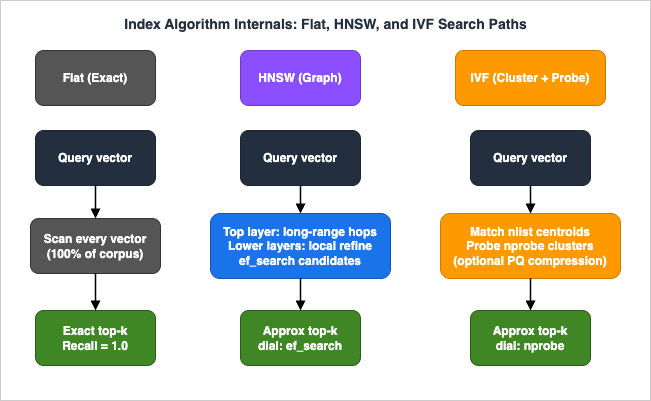

Internal structure and search path of Flat, HNSW, and IVF vector indexes

3.1 Flat — exhaustive scan

Structure: none beyond the raw vectors, stored contiguously (often at full 32-bit float precision).

Search path: compute the distance from the query to every stored vector, maintain a running top-k heap, return it. The query touches 100% of the data.

Characteristics:

Recall: exact (1.0). This is the reference against which every ANN index's recall is measured.
Latency: grows linearly with corpus size. Fine for small sets, prohibitive for large ones.
Memory: stores every full-precision vector; no graph or codebook overhead, but no compression either.
Build/update: trivial — inserting a vector is just appending it. No index to rebuild.

Flat is the right default for small corpora and the correct baseline for measuring any ANN index you deploy: run a sample of queries against Flat to get ground truth, then measure your ANN recall against it.

3.2 HNSW — Hierarchical Navigable Small World graphs

HNSW is the most widely deployed ANN algorithm on AWS; every vector-capable service here supports it.

Structure: a multi-layer proximity graph. Each vector is a node. The bottom layer connects every node to its nearby neighbors, forming a dense "small world" graph where any two points are reachable in few hops. Higher layers contain progressively fewer nodes, each holding long-range links that act like an express network. A node's presence in the upper layers is decided probabilistically at insert time.

Search path: start at an entry point in the top (sparsest) layer and greedily walk toward the query — repeatedly moving to the neighbor closest to the query vector. When no neighbor in the current layer is closer, drop down a layer and continue. The top layers cover distance quickly; the bottom layer refines to the true neighborhood. The search maintains a dynamic candidate list whose size controls how thoroughly the neighborhood is explored.

Parameters (the same three concepts recur across every service, sometimes with different names):

m (a.k.a. M) — the maximum number of neighbor links each node keeps per layer. Higher m builds a denser graph: better recall, but more memory and slower builds. A common starting point is 16.
ef_construction (a.k.a. EF_CONSTRUCTION) — the size of the candidate list used while building the graph. Higher values produce a higher-quality graph at the cost of longer index build time. It is set at build time and cannot be changed without rebuilding.
ef_search (a.k.a. EF_RUNTIME, ef) — the size of the candidate list used at query time. This is the primary recall-vs-latency dial and, importantly, it is usually tunable per query without rebuilding. Raising it explores more of the graph: higher recall, higher latency.

Characteristics:

Recall: excellent and finely tunable via ef_search.
Latency: low and roughly logarithmic in corpus size — HNSW's headline advantage.
Memory: high. The graph and its full-precision vectors must stay resident in memory (or its cost-tiered equivalent) for good performance; graph links add overhead on top of the vectors themselves. This is HNSW's main cost and the reason quantization (Section 4) matters at scale.
Build/update: inserts are supported incrementally, but heavy deletes and overwrites degrade HNSW. Removed vectors often leave the graph structure behind (a form of tombstoning), which inflates memory and erodes recall over time until the index is rebuilt — the "index bloat" failure mode in Section 10.

3.3 IVF — Inverted File (cluster-and-probe)

IVF trades some of HNSW's recall smoothness for dramatically lower memory, which is why it appears at very large scale.

Structure: during a training step, run k-means over a representative sample to partition the space into nlist clusters (Voronoi cells), each with a centroid. Every vector is then assigned to its nearest centroid, producing an inverted list per cluster (cluster → the vectors that belong to it).

Search path: compare the query only to the nlist centroids, pick the nprobe nearest clusters, and scan only the vectors in those clusters. The rest of the corpus is never touched. nprobe = 1 is fastest and lowest-recall; increasing nprobe searches more clusters, raising recall toward exhaustive.

Parameters:

nlist — number of clusters. More clusters → smaller, more selective cells → less work per probe, but the query must find the right cells. Chosen relative to corpus size.
nprobe — number of clusters probed per query. The primary recall-vs-latency dial, tunable per query.

IVF with Product Quantization (IVF-PQ): IVF is frequently paired with product quantization, which splits each vector into sub-vectors and replaces each with the ID of the nearest entry in a learned codebook. This compresses vectors by an order of magnitude, slashing memory — the key reason IVF-PQ scales to enormous corpora — at the cost of some recall, usually recovered by re-ranking the shortlist with full-precision vectors.

Characteristics:

Recall: tunable via nprobe; typically a notch below HNSW at equal latency, and lower still with aggressive PQ unless you re-rank.
Latency: low once trained; you scan a fraction of the data.
Memory: low, especially with PQ — its decisive advantage over HNSW at scale.
Build/update: requires training on representative data before you can index, and the trained partitioning assumes the data distribution is stable. If the distribution shifts substantially, cluster quality (and recall) drifts and you retrain. This training requirement is why some managed/serverless offerings do not expose IVF at all.

3.4 Reading the trade-off

* You can sort the table by clicking on the column name.

Property	Flat (exact)	HNSW	IVF (± PQ)
Recall	Exact (1.0)	Excellent, tunable (`ef_search`)	Good, tunable (`nprobe`); lower with PQ unless re-ranked
Query latency	Linear in corpus size	Low, ~logarithmic	Low once trained
Memory footprint	Full-precision vectors only	High (graph + resident vectors)	Low, very low with PQ
Build cost	None	Moderate; `ef_construction` sets quality	Training required up front
Updates	Trivial	Incremental; degrades on heavy delete/overwrite	Incremental; retrain on distribution shift
Best fit	Small corpora; recall ground truth	Low-latency ANN at moderate–large scale	Very large corpora; memory-constrained

The mental model to carry into the service sections: ef_search (HNSW) and nprobe (IVF) are the runtime recall dials; m / ef_construction (HNSW) and nlist / training (IVF) are the build-time structure decisions; and quantization is how you buy back memory when the full-precision footprint gets too large.

4. Amazon OpenSearch Service and Serverless

OpenSearch is the most configurable vector store on AWS and the one that exposes the algorithm internals from Section 3 most directly. It comes in two operational forms: Amazon OpenSearch Service (managed domains / clusters you size) and Amazon OpenSearch Serverless (a serverless collection that scales itself).

4.1 The k-NN plugin, engines, and algorithms

Vector search in OpenSearch is provided by the k-NN plugin, which stores embeddings in a knn_vector field and can search them three ways: approximate k-NN (the ANN path), script score (exact), and Painless extensions (exact). The approximate path is backed by one of three underlying libraries — called engines — each supporting different algorithms:

Faiss — supports HNSW and IVF (with and without product quantization). The most capable engine; the one to pick when you want IVF or PQ.
Lucene — supports HNSW only, with native filter-while-search.
NMSLIB — supports HNSW only. This is the original engine and is now legacy — newer OpenSearch versions steer new indexes toward Faiss, so treat NMSLIB as something you may inherit, not something to choose for a new build.

A knn_vector field supports high dimensionality (up to 16,000 for the native engines), which comfortably covers every current embedding model. You configure the algorithm in the field's method block:

PUT /my-vector-index
{
  "settings": {
    "index": {
      "knn": true,
      "knn.algo_param.ef_search": 100
    }
  },
  "mappings": {
    "properties": {
      "embedding": {
        "type": "knn_vector",
        "dimension": 1024,
        "space_type": "cosinesimil",
        "method": {
          "name": "hnsw",
          "engine": "faiss",
          "parameters": {
            "ef_construction": 256,
            "m": 16
          }
        }
      }
    }
  }
}

Here space_type sets the metric (l2, innerproduct, cosinesimil), the method block sets the algorithm and its build-time parameters (m, ef_construction), and the index-level knn.algo_param.ef_search sets the query-time recall dial. These map one-to-one onto the HNSW concepts from Section 3.2.

4.2 Quantization: buying back memory

Because HNSW keeps vectors resident, memory is the constraint that grows with your corpus. OpenSearch offers several quantization options to shrink the footprint:

FP16 scalar quantization (SQfp16) — stores each dimension as a 16-bit float instead of 32-bit, halving memory, with clipping to keep values in range. Configured with an encoder of type fp16 on a Faiss HNSW field.
Byte / scalar quantization — one byte per dimension (available with the Lucene engine), reducing storage and query latency with minimal recall impact.
Product quantization — the aggressive, codebook-based compression used with Faiss IVF for the largest corpora.
Binary vectors — one bit per dimension, the most extreme compression, typically paired with a full-precision re-rank of the shortlist to recover recall.
Disk-based vector search — keeps compressed vectors in memory and full-precision vectors on disk, cutting the memory bill for low-memory, cost-sensitive workloads.

The design pattern is consistent: quantize to fit the working set into memory, then re-rank the shortlist with higher precision to recover the recall you gave up.

4.3 Filtering and hybrid search

Two capabilities make OpenSearch the choice when retrieval is more than pure vector similarity:

Efficient (pre-)filtering. OpenSearch can apply a metadata filter before the nearest-neighbor search (pre-filtering), so the ANN search runs only over the surviving candidates. Faiss gained efficient filtering so you get this with a scalable engine; Lucene offers filter-while-search that automatically picks pre-filtering, post-filtering, or exact k-NN depending on selectivity. This directly addresses the filter-performance failure mode in Section 10.2 — naive post-filtering searches first and then discards, which can leave you with fewer than k results.
Hybrid search. OpenSearch can run a lexical (BM25 keyword) query and a k-NN (semantic) query together and combine the normalized scores. Pure semantic search is weak at exact-term matching — product codes, drug names, legal citations, error identifiers — where the right document must contain a specific token. Hybrid search recovers those matches. (The mechanics of tuning hybrid search are a retrieval-quality topic covered in the companion Knowledge Bases retrieval-quality guide; here it is one reason to prefer OpenSearch.)

4.4 Managed domains vs Serverless — the operational fork

The two forms differ in more than billing model, and the difference constrains your algorithm choices:

OpenSearch Service (managed domain/cluster) gives you full control: all three engines, IVF (including PQ) via the training APIs, and the ability to size and tune nodes. You operate the cluster. It integrates with Amazon Bedrock Knowledge Bases as a managed-cluster vector store.
OpenSearch Serverless (vector search collection) removes sizing and tuning: it scales compute and storage independently and automatically. The trade-off is reduced algorithm surface — Serverless standardizes on Faiss HNSW and does not expose the training APIs, so IVF is not available on Serverless. Newer collections use the "next-generation" vector collection type (the older "classic" collections still support Faiss 16-bit scalar quantization, binary vectors, and disk-based search). Serverless is the store Bedrock Knowledge Bases can create for you automatically.

Choose OpenSearch when you need hybrid (lexical + semantic) search, rich metadata pre-filtering, the widest algorithm/quantization control (managed domains), or you are already running OpenSearch for logs/search and want to consolidate. Lean Serverless when you want those retrieval capabilities without operating a cluster and HNSW is sufficient; lean a managed domain when you specifically need IVF/PQ or fine node-level control.

5. Amazon Aurora PostgreSQL with pgvector

If your application already lives in a relational database, the most consequential fact in this guide may be that you can add vector search to it without adopting a separate system. pgvector is a PostgreSQL extension that adds a vector data type and nearest-neighbor operators, available on Amazon Aurora PostgreSQL-Compatible Edition (and Amazon RDS for PostgreSQL).

5.1 The extension, versions, and types

You enable it with CREATE EXTENSION vector;. Aurora tracks the upstream project closely — pgvector 0.8.x is available on current Aurora PostgreSQL minor versions (0.8.0 from PostgreSQL 13.20+/14.17+/15.12+/16.8+/17.4+, with newer minors shipping later patch releases); check the Aurora PostgreSQL extensions reference for the exact version on your engine version. Beyond the core vector type, recent pgvector adds halfvec (2-byte half-precision, halving storage), bit (for binary quantization), and sparsevec.

Bedrock Knowledge Bases requires pgvector 0.5.0 or later because that is the version that introduced HNSW indexing; earlier versions had only IVFFlat.

5.2 Index types and metrics

pgvector supports both index algorithms from Section 3, plus exact search:

Exact search — no index; a sequential scan computes true nearest neighbors. Correct for small tables, and the recall baseline for the others.
IVFFlat — the inverted-file algorithm. Build parameter lists (= nlist), query parameter probes (= nprobe). IVFFlat should be built after the table has representative data, because it clusters the existing rows.
HNSW — the graph algorithm. Build parameters m (default 16) and ef_construction (pgvector default 64; AWS commonly recommends 128), query parameter ef_search (pgvector default 40, set per session with SET hnsw.ef_search). The default ef_search of 40 is frequently too low for production recall — tune it, don't inherit it.

Distance is chosen via the operator and the matching operator class:

<-> L2 distance (vector_l2_ops)
<=> cosine distance (vector_cosine_ops)
<#> (negative) inner product (vector_ip_ops)
<~> Hamming and Jaccard distance on bit vectors, for binary-quantized retrieval

-- Enable the extension and create a table with a 1024-dim column
CREATE EXTENSION IF NOT EXISTS vector;

CREATE TABLE documents (
  id         bigint PRIMARY KEY,
  tenant_id  text NOT NULL,
  content    text,
  embedding  vector(1024)
);

-- HNSW index for cosine distance
CREATE INDEX ON documents
  USING hnsw (embedding vector_cosine_ops)
  WITH (m = 16, ef_construction = 128);

-- Tune the query-time recall dial for this session
SET hnsw.ef_search = 100;

-- Vector search combined with a metadata predicate, in one query
SELECT id, content
FROM documents
WHERE tenant_id = 'acme'
ORDER BY embedding <=> '[...query embedding...]'
LIMIT 10;

5.3 The SQL-integration advantage

The last query above is the whole point of pgvector: the vector similarity ordering and the metadata predicate (WHERE tenant_id = 'acme') execute together in a single ACID query. You get exact, index-backed metadata filtering, joins to related relational data, transactional consistency between your embeddings and your business data, and natural per-tenant isolation via row predicates — all without a second datastore to keep in sync. For teams whose source of truth is already PostgreSQL, this eliminates an entire ingestion-and-reconciliation pipeline.

pgvector also supports the memory-saving patterns from Section 4. Binary quantization with two-stage retrieval narrows candidates on tiny binary vectors (Hamming distance) and then re-ranks the shortlist by full-precision cosine distance — recovering most of the recall lost to quantization. Aurora Optimized Reads extends the effective working-set memory for large HNSW indexes.

-- Two-stage retrieval: coarse pass on binary-quantized vectors, cosine re-rank
SELECT id, content
FROM (
  SELECT id, content, embedding
  FROM documents
  WHERE tenant_id = 'acme'
  ORDER BY binary_quantize(embedding)::bit(1024)
           <~> binary_quantize('[...query embedding...]')
  LIMIT 100
) candidates
ORDER BY embedding <=> '[...query embedding...]'
LIMIT 10;

Choose Aurora pgvector when PostgreSQL is already your system of record, when you need vector similarity and structured predicates (or joins) evaluated together with transactional consistency, or when per-tenant isolation maps naturally to row-level filtering. Its practical ceiling is instance-dependent (millions of vectors rather than billions); at very large scale, a purpose-built engine or a cost-tiered store fits better.

6. Amazon MemoryDB Vector Search

Amazon MemoryDB is a durable, in-memory database compatible with the Valkey and Redis OSS APIs. Its vector search extends that in-memory engine, which is why its defining characteristic is latency: because vectors and the index live in memory and index updates apply in single-digit milliseconds, MemoryDB targets the lowest-latency, freshest-index end of the spectrum, achieving single-digit-millisecond p99 query times at high recall.

6.1 Algorithms and parameters

MemoryDB offers exactly two index algorithms, mapping straight onto Section 3:

FLAT — brute-force exact search. The documentation positions it for smaller stores where a linear scan stays fast enough, since query run time grows steeply as the index gets large.
HNSW — the graph algorithm for larger stores, controlled by three parameters: M, EF_CONSTRUCTION (both fixed at index-creation time), and EF_RUNTIME (a default set at creation that can be overridden on any individual query). An optional INITIAL_CAP pre-allocates index memory to reduce management overhead and speed ingestion.

Distance metrics are configurable: cosine, dot product (inner product), and Euclidean (L2). Vectors are stored as JSON or hash types and searched with the FT.SEARCH and FT.AGGREGATE commands, which support pre-filtering by combining vector queries with boolean predicates over other fields.

FT.CREATE idx:docs ON JSON PREFIX 1 doc: SCHEMA
  $.embedding AS embedding VECTOR HNSW 6
    TYPE FLOAT32 DIM 1024 DISTANCE_METRIC COSINE
    M 16 EF_CONSTRUCTION 128
  $.tenant AS tenant TAG

The same three HNSW knobs appear again — M, EF_CONSTRUCTION, and the query-time EF_RUNTIME — reinforcing that the algorithm, not the product, dictates the tuning surface.

6.2 Where MemoryDB fits, and a critical integration caveat

MemoryDB's in-memory nature makes it the strongest fit for real-time, latency-critical retrieval: semantic caching for LLM applications (matching a new prompt against recent ones), real-time recommendation and personalization, fraud/anomaly detection, and RAG paths where retrieval latency is on the user's critical path. It scales to sizeable clusters, and its durability (it is a database, not just a cache) means you can store embeddings alongside your primary data.

The same HNSW caveat applies: heavy deletes and overwrites can inflate index memory and degrade recall, and the fix is reindexing (Section 10.3).

The critical caveat for selection: MemoryDB is not one of the vector stores that Amazon Bedrock Knowledge Bases can use (Section 8). If you want a fully managed KB to own ingestion and retrieval, MemoryDB is not an option — you would build the retrieval path yourself against MemoryDB, or use MemoryDB for a latency-sensitive layer (such as a semantic cache) alongside a KB backed by a supported store. This single fact frequently decides MemoryDB in or out of a design.

7. Amazon S3 Vectors and Where It Fits

Amazon S3 Vectors is the first cloud object storage with native support for storing and querying vectors, generally available since late 2025. It occupies the opposite corner of the design space from MemoryDB: where MemoryDB optimizes for the lowest latency by keeping everything in memory, S3 Vectors optimizes for elastic, durable, cost-efficient storage at massive scale with a fully serverless model — no infrastructure to provision, dedicated s3vectors APIs to put and query vectors, and durability and elasticity inherited from Amazon S3.

Its scale and operational profile are what define its niche: a single vector index holds up to 2 billion vectors, a vector bucket up to 10,000 indexes, with per-vector dimensions from 1 to 4,096, cosine or Euclidean distance, and metadata filtering. Query latency is designed for interactive-but-not-hot access — under a second for infrequent queries, around 100 milliseconds for more frequent ones — which places it at the large, cost-sensitive, moderate-latency end of the spectrum rather than the real-time end. It integrates with Bedrock Knowledge Bases as a native vector store.

Because a dedicated deep dive already exists, this guide deliberately keeps S3 Vectors to its position in the selection landscape and delegates the specifics — the exact limits, the frequency-dependent latency behavior, immutable index configuration, the semantic-only (no keyword) search model, and hot/cold tiered designs that pair S3 Vectors with OpenSearch — to Amazon S3 Vectors Design Decision Guide. The one-line placement: reach for S3 Vectors when the corpus is large, access is infrequent or cost-dominated, and around-100-millisecond latency is acceptable; reach elsewhere when you need the lowest latency (MemoryDB), the richest filtering/hybrid search (OpenSearch), or transactional SQL integration (Aurora).

Amazon Neptune Analytics rounds out the picture for a different shape of problem: it is a graph analytics engine with a native HNSW vector index (L2 distance, very high dimensionality), searchable directly from openCypher, so you can combine vector similarity with graph traversals in one query. That is the GraphRAG pattern — retrieving context by relationship (lineage, provenance, connection) as well as by similarity — and its mechanics are covered in GraphRAG Architecture on AWS with Amazon Neptune and Amazon Bedrock. Choose it when your retrieval needs to traverse a knowledge graph, not just rank by distance.

8. Knowledge Bases Integration and the RAG Stack

For many teams the vector store is not chosen in isolation — it is chosen as the backing store for Amazon Bedrock Knowledge Bases, which automates the RAG ingestion pipeline (parsing, chunking, embedding generation, indexing) and the retrieval APIs on top of whichever store you configure. So "which store integrates with Knowledge Bases, and with what consequences" is itself a primary selection axis.

A scope note first: since the general availability of Amazon Bedrock Managed Knowledge Base (June 2026), Knowledge Bases comes in two forms. In a managed knowledge base, Bedrock owns the embedding model, the vector storage, and the retrieval infrastructure end to end — you never select a vector store, so the selection question this article answers does not arise there. Everything in this section describes the customer-managed knowledge base, where you bring and configure one of the stores below and the store's properties remain your responsibility. If a fully managed retrieval stack fits your requirements, evaluate the managed form first; if you need control over the store — hybrid search tuning, SQL co-location, cost-tiered storage, graph retrieval — the customer-managed form is where this guide applies.

8.1 The supported vector stores

Knowledge Bases writes and manages embeddings in a vector store you specify via its storage configuration. The supported store types are:

Amazon OpenSearch Serverless (and it can create one for you automatically)
Amazon OpenSearch Service managed cluster
Amazon Aurora PostgreSQL (via the RDS configuration)
Amazon Neptune Analytics (for GraphRAG)
Amazon S3 Vectors
Pinecone, MongoDB Atlas, and Redis Enterprise Cloud (third-party)

The consequence for selection is sharp: Amazon MemoryDB is not in this list. MemoryDB's vector search is a powerful standalone capability, but if Knowledge Bases integration is a hard requirement, MemoryDB is off the table for that role — a point worth confirming early, because it is easy to assume "AWS vector store" means "KB-compatible."

The store you pick still carries all its properties into the KB: choose OpenSearch for hybrid search and filtering, Aurora for SQL-integrated filtering and transactional consistency, S3 Vectors for cost-efficient scale, Neptune Analytics for graph retrieval. The KB abstracts the pipeline, not the store's capabilities.

8.2 Embedding models and dimensions

The KB (or your own pipeline) needs an embedding model, and the model's output dimension must match the vector index's configured dimension. On Amazon Bedrock the representative choices are:

Amazon Titan Text Embeddings V2 (amazon.titan-embed-text-v2:0) — output dimension 1024 (default), 512, or 256, up to 8,192 input tokens, multilingual support (100+ languages, listed as preview in the current AWS documentation), and optional binary embeddings. Its selectable dimension is a genuine tuning lever: AWS reports that reducing from 1024 to 512 dimensions retains roughly 99% of retrieval accuracy, and 256 dimensions retains roughly 97% — so you can cut vector storage substantially while keeping most of the accuracy (a Matryoshka-style truncation trade-off).
Cohere Embed (English and Multilingual v3) — 1024-dimensional vectors with binary-vector support; the multilingual variant covers 100+ languages and requires an input_type parameter per call. Cohere's newer Embed generation extends this to unified multimodal (text + image) embeddings.

Two honesty notes worth carrying into a design. First, Anthropic's Claude models do not provide an embeddings API — Claude is a generation (and reasoning) model; embeddings for your RAG index come from Bedrock models like Titan or Cohere, or from third-party embedding providers, not from Claude. Second, because the index dimension is fixed at creation and tied to the model, switching embedding models later generally means re-embedding the corpus and rebuilding the index — choose the model (and dimension) with the same care as the store.

For the current, authoritative list of embedding models and their dimensions, consult the Bedrock model documentation rather than any snapshot — the lineup changes often. The mechanics of chunking, hybrid search, metadata filtering, and reranking inside a Knowledge Base are the subject of the companion guide, Amazon Bedrock Knowledge Bases Retrieval Quality Engineering, and are out of scope here.

9. The Decision Flow

With the algorithms and services established, selection reduces to a small set of questions asked in roughly this order. The flow below encodes them; the prose after it explains the branch points.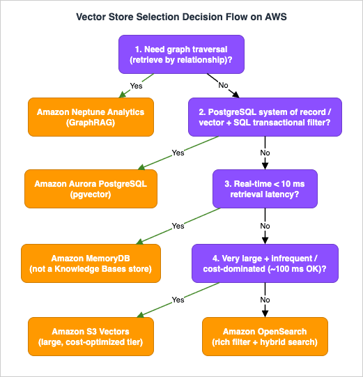

Decision flow for selecting a vector store on AWS

Do you need graph traversal (retrieval by relationship, not just similarity)? If yes → Neptune Analytics (GraphRAG). If no, continue.
Is PostgreSQL already your system of record, or do you need vector similarity and structured predicates/joins evaluated together with transactional consistency? If yes → Aurora PostgreSQL with pgvector. This is often the lowest-friction choice for teams already relational, and it gives exact metadata filtering in the same query as the vector search.
Is retrieval latency on the user's critical path — sub-10-millisecond, real-time (semantic cache, live recommendations)? If yes → MemoryDB (remembering it is not a Knowledge Bases store, so you own the retrieval path).
Is the corpus very large and access infrequent or cost-dominated, with ~100-millisecond latency acceptable? If yes → S3 Vectors (see the dedicated guide; consider a hot/cold tier with OpenSearch for the frequently-queried subset).
Otherwise — you need rich filtering, hybrid (lexical + semantic) search, or the widest algorithm/quantization control → OpenSearch. Pick Serverless to avoid operating a cluster (Faiss HNSW, no IVF), or a managed domain when you specifically need IVF/PQ or node-level tuning.

Two cross-cutting inputs modulate every branch:

Do you want a managed Knowledge Base to own ingestion and retrieval? If yes, restrict to KB-supported stores (Section 8.1) — which removes MemoryDB from consideration for that role.
Scale and precision set the index algorithm inside the chosen store. Small corpus → Flat (exact, no tuning, perfect recall). Moderate-to-large with low-latency needs → HNSW, tuned via ef_search. Very large and memory-constrained → IVF/IVF-PQ where available (Faiss on OpenSearch managed domains, or IVFFlat on Aurora), tuned via nprobe. Update frequency matters too: workloads with heavy deletes/overwrites need a reindexing plan regardless of store, because HNSW degrades under churn.

The decision is never store-only or algorithm-only; it is the pair. "Aurora with HNSW at ef_search = 100," "OpenSearch Serverless with Faiss HNSW and FP16 quantization," "S3 Vectors for the cold tier plus OpenSearch HNSW for the hot subset" — these are the shape of a real answer.

10. Diagnostics: Recall Degradation and Filter Performance

Three failure modes account for most production vector-search incidents. Each has a recognizable symptom, a small set of root causes, and a direct remedy. The unifying discipline is that you must measure recall against exact (Flat) ground truth rather than eyeball result quality — Section 2.2 exists partly to give you that baseline.

10.1 Recall degradation — the right result is missing from the top-k

Symptom: a query that obviously should return a particular document doesn't, or answer quality quietly drops after a change.

Root causes and fixes:

Runtime recall dial too low. The most common cause. Raise ef_search (HNSW) or nprobe (IVF). Recall improves at some latency cost; find the operating point by sweeping the value and measuring recall against Flat. Remember pgvector's hnsw.ef_search defaults to 40, which is often too low.
Metric mismatch. The index metric doesn't match how the embeddings were trained (e.g., cosine index but inner-product embeddings), or the embeddings aren't normalized when the metric assumes unit vectors. Align the space_type / operator class with the model, and normalize if required.
Over-aggressive quantization. Binary or heavy product quantization discarded too much precision. Add a full-precision re-rank stage over the shortlist (the two-stage pattern in Sections 4.2 and 5.3), or reduce the compression level.
Dimension mismatch or wrong model. The stored dimension doesn't match the query model's output, or the corpus was embedded with a different model than the query. Re-embed consistently.

10.2 Filter performance — slow or under-filled results when a metadata filter is applied

Symptom: adding a WHERE/filter clause makes queries much slower, or returns fewer than k results.

Root causes and fixes:

Post-filtering. The engine ran the ANN search first and then discarded non-matching results, leaving fewer than k — especially when the filter is highly selective. Switch to a pre-filtering / filter-while-search path: OpenSearch's efficient filtering (Faiss) or filter-while-search (Lucene); Aurora's SQL WHERE with an appropriate index; MemoryDB's FT.SEARCH pre-filter. Pre-filtering searches only the surviving candidates.
Metadata not designed for filtering. High-cardinality or poorly-typed metadata makes filters expensive. Design filterable fields deliberately (tenant, department, language, time bucket) and keep them in the filterable metadata budget the store defines.
Selectivity too high for ANN. When a filter leaves very few candidates, exact search over that subset can beat ANN. Lucene's filter-while-search picks this automatically; elsewhere, over-fetch and re-rank, or fall back to exact for the filtered subset.

The structural point from Section 4.3: the ability to pre-filter efficiently is a store-selection criterion, not just a tuning detail. If precise, high-selectivity metadata filtering is central to your workload, that argues for OpenSearch or Aurora over stores with weaker filter integration.

10.3 Index bloat — memory growth and recall decay after heavy updates

Symptom: an HNSW-backed index that has taken many deletes and overwrites uses more memory than expected, gets slower, and loses recall over time.

Root causes and fixes:

HNSW tombstoning. Deleting or overwriting vectors in an HNSW graph often leaves structure behind rather than truly removing it, inflating memory and degrading the graph's navigability. This is inherent to the algorithm, not a specific product's bug.
Remedies: reindex/rebuild to restore optimal memory and recall — the primary fix. Reduce churn by batching updates. Pre-allocate with INITIAL_CAP (MemoryDB) when you can estimate final size. For write-heavy workloads generally, favor a store and pattern that tolerate rebuilds (e.g., blue/green index swaps) and schedule periodic reindexing rather than letting the graph decay indefinitely.

Across all three failure modes, the same instrumentation pays off: keep a held-out query set with known-correct (exact) answers, compute recall@k after every configuration change, and watch the recall-versus-latency curve rather than any single number. That is what turns vector-store operation from guesswork into engineering.

11. Frequently Asked Questions

Is a vector database different from a vector index?
An index is the searchable structure (Flat, HNSW, IVF) built over your embeddings; a vector store/database is the system that hosts one or more such indexes and provides ingestion, querying, durability, and often metadata filtering. On AWS the "store" is the service (OpenSearch, Aurora, MemoryDB, S3 Vectors, Neptune Analytics) and the "index algorithm" is what you configure inside it.

HNSW or IVF — which should I use?
Default to HNSW for low-latency ANN at moderate-to-large scale; it is broadly available and finely tunable via ef_search. Reach for IVF (especially IVF-PQ) at very large scale when memory is the binding constraint and you can afford the training step — but note IVF is not available everywhere (for example, OpenSearch Serverless is HNSW-only). For small corpora, prefer neither: use exact Flat search.

When is exact search actually the right choice?
When the corpus is small enough that a full scan is fast — typically corpora in the tens of thousands of vectors, and often well beyond for per-tenant subsets; benchmark your own latency budget rather than relying on a fixed threshold. Flat gives perfect recall with zero tuning, and it is always the correct baseline for measuring an ANN index's recall.

Can I use Amazon MemoryDB with Amazon Bedrock Knowledge Bases?
No. MemoryDB is not among the customer-managed Knowledge Bases vector stores (which include OpenSearch Serverless and managed clusters, Aurora PostgreSQL, Neptune Analytics, S3 Vectors, Pinecone, MongoDB Atlas, and Redis Enterprise Cloud). Use MemoryDB standalone for latency-critical retrieval, or alongside a KB backed by a supported store.

Do Claude models generate embeddings?
No. Anthropic's Claude models are for generation and reasoning; they do not expose an embeddings API. Generate embeddings with Amazon Bedrock models such as Amazon Titan Text Embeddings V2 or Cohere Embed, or a third-party embedding provider.

Does the embedding dimension matter for the vector store?
Yes, in two ways. The index is created with a fixed dimension that must match the model's output, so changing models or dimensions later means re-embedding and rebuilding. And smaller dimensions cut storage and search cost: Titan Text Embeddings V2 lets you pick 256/512/1024, retaining roughly 97%/99%/100% of retrieval accuracy respectively — a lever worth pulling when storage or latency is tight.

How do I fix a query that suddenly returns worse results?
Work Section 10.1 in order: raise the runtime recall dial (ef_search/nprobe), verify the distance metric and normalization match the model, check for over-aggressive quantization (add a re-rank), and confirm the dimension and embedding model are consistent between indexing and querying. Always measure recall against exact ground truth rather than trusting impressions.

What is the fastest vector search option on AWS?
For lowest query latency, Amazon MemoryDB — because vectors and index live in memory, it targets single-digit-millisecond p99 at high recall. That speed is the reason to choose it, and the reason it is not the right home for very large, cost-sensitive, or infrequently-queried corpora, where S3 Vectors fits better.

12. Summary

Choosing a vector store on AWS is a two-part decision, and the two parts are inseparable. The store — OpenSearch, Aurora pgvector, MemoryDB, S3 Vectors, or Neptune Analytics — is chosen from the shape of your workload: graph traversal points to Neptune Analytics; a relational system of record and transactional filtering points to Aurora; sub-10-millisecond real-time retrieval points to MemoryDB; very large, cost-dominated corpora point to S3 Vectors; and rich filtering plus hybrid search points to OpenSearch. A managed Knowledge Base narrows the field to KB-supported stores, which notably excludes MemoryDB.

The index algorithm — Flat, HNSW, or IVF — is chosen from scale and precision, and it is where the tuning lives. Flat gives exact recall for small corpora and the ground truth for everything else. HNSW gives low-latency ANN tuned by ef_search, at the cost of resident memory that quantization can reclaim. IVF (and IVF-PQ) scales furthest on the least memory, at the cost of a training step and availability limited to certain stores. The same three concepts recur under different names in every service — the neighbor count, the build-time candidate list, and the query-time candidate list for HNSW; the cluster count and probe count for IVF — so once you can read one, you can read them all.

The engineering discipline that ties it together is measuring recall against exact ground truth and watching the recall-versus-latency curve as you tune. Do that, design your metadata for pre-filtering, and plan for reindexing under churn, and vector search becomes a predictable engineering problem rather than a source of mysterious quality regressions. From here, the natural next steps are tuning retrieval quality inside a Knowledge Base — chunking, hybrid search, reranking — in Amazon Bedrock Knowledge Bases Retrieval Quality Engineering, and, for the lowest-latency layer, designing an embedding-based semantic cache for LLM applications on AWS.

13. References

References:
Tech Blog with curated related content

Written by Hidekazu Konishi