Amazon DynamoDB Capacity and Global Tables Guide - Capacity Modes, Auto Scaling, Warm Throughput, and Multi-Region Design
First Published:
Last Updated:
This guide is the operations companion to the DynamoDB design articles on this site. It deliberately does not re-teach key design, secondary indexes, or single-table modeling. For partition key and index design — including the key-design remedies for hot partitions such as write sharding and read sharding — see the Amazon DynamoDB Key Design and GSI/LSI Dictionary; for modeling many entities in one table, see the Amazon DynamoDB Single Table Design Guide. For when each capability shipped, the AWS History and Timeline regarding Amazon DynamoDB is the reference, and the AWS Database Glossary defines the terms used here.
Here, the subject is throughput: how the two capacity modes actually behave, how auto scaling and warm throughput shape what your table can absorb, why a table throttles even when it looks under-provisioned, and how global tables replicate, fail over, and force a different way of thinking about capacity. The goal is that you can decide and operate — not just describe — DynamoDB at scale and across Regions.
Scope note. This is an operations guide, not a cost guide. The choice between on-demand and provisioned capacity is frequently framed as "which is cheaper," but that framing leads to brittle decisions. Throughput characteristics — predictability of traffic, operational model, and spike tolerance — are what should drive the choice, and those are what this article uses. Cost is real and matters to a final design, but pricing changes often and is per-Region, so cost is described qualitatively and you should confirm numbers on the official Amazon DynamoDB pricing page. Every quantitative limit cited below was verified against AWS documentation; always confirm current quotas in the Service Quotas console for your account and Region.
A note on units. DynamoDB measures throughput in capacity units. One read capacity unit (RCU) is one strongly consistent read per second for an item up to 4 KB (or two eventually consistent reads); one write capacity unit (WCU) is one write per second for an item up to 1 KB. On-demand tables use the equivalent read request units (RRU) and write request units (WRU), billed per request. The same per-item sizing rules apply in both modes — a 5 KB item read strongly costs 2 RCUs, an 8 KB write costs 8 WCUs — so the difference between the modes is how capacity is managed and charged, not how an individual operation is metered.
1. The Capacity Problem in One Picture
DynamoDB presents a simple API and hides an enormous amount of distributed-systems machinery. To operate it well, you need a mental model of three layers and how they interact:- The mode layer decides whether you manage capacity (provisioned) or DynamoDB does (on-demand). This sets the ceiling and the billing model.
- The elasticity layer — auto scaling for provisioned tables, automatic scaling for on-demand, and warm throughput on top of both — decides how fast the ceiling can move and how much the table can absorb right now.
- The partition layer decides what physically happens to a request. Every table is split into partitions, each with hard per-partition throughput limits, and most "mysterious" throttling originates here rather than at the table level.
Multi-Region adds a fourth dimension on top of all three: global tables replicate your data across Regions, which changes how writes are acknowledged, how conflicts resolve, and — crucially — how much capacity each Region must be prepared to serve when another Region's traffic suddenly arrives.
The rest of this guide walks these layers from the top down, then assembles them into a multi-Region architecture. We start with the mode choice because it constrains everything below it — but we keep it short, because the depth is in the layers underneath.
2. Capacity Modes: On-Demand vs Provisioned
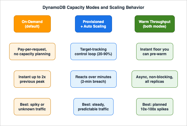
Every DynamoDB table is created in one of two throughput modes, and the choice governs how capacity is managed and billed.On-demand mode is the default and the recommended option for most workloads. You do not specify throughput; DynamoDB scales automatically and you pay per request. A new on-demand table can instantly sustain up to 4,000 writes and 12,000 reads per second, and from there it tracks your traffic. It is the natural fit for serverless applications, unpredictable or spiky traffic, new tables with no usage history, and any workload where you would rather not own a capacity-planning loop.
Provisioned mode requires you to specify read and write capacity in advance, and you are billed for what you provision — not what you consume. It suits steady, predictable workloads where you can forecast demand and want a firm rate ceiling for cost governance. Provisioned mode is rarely used bare; it is almost always paired with auto scaling (Section 3) so the provisioned numbers track demand within bounds you set.
The decision is not about price. It is about three properties:
- Traffic predictability. Predictable, steady traffic can be provisioned accurately; spiky or unknown traffic cannot, and over-provisioning to cover the spikes wastes capacity while under-provisioning throttles. On-demand removes the forecast from the equation.
- Operational model. Provisioned mode is a control loop you own — targets, alarms, minimums, maximums. On-demand is managed for you. Teams without capacity to run that loop should default to on-demand.
- Spike tolerance. On-demand absorbs spikes up to a structural limit (double the previous peak, discussed below) with no configuration. Provisioned mode absorbs spikes only within burst capacity and the speed of auto scaling.
The figure below summarizes the two modes and the elasticity features layered on each.
2.1 On-demand scaling and the "double the previous peak" rule
On-demand is not infinite-from-zero. It scales relative to the highest throughput your table has previously reached — its previous peak. On-demand instantly accommodates up to double the previous peak at any time. The mechanic is worth stating precisely because it is the root cause of a class of launch-day throttling:Suppose a table's traffic oscillates between 25,000 and 50,000 strongly consistent reads per second. The previous peak is 50,000, so on-demand will instantly serve up to 100,000 reads per second. If the workload then sustains 100,000, that becomes the new previous peak, and subsequent traffic can reach 200,000. DynamoDB allocates more capacity automatically as traffic grows — but if you exceed double the previous peak within 30 minutes, throttling can occur. The guidance is to either pre-warm the table (Section 4) or spread traffic growth over at least 30 minutes before driving more than double the last peak. There is no 30-minute restriction as long as you stay within double the previous peak.
A new on-demand table starts with a baseline of 4,000 writes and 12,000 reads per second, so small and moderate launches are covered without any action. It is large step-changes — a flash sale, a marketing blast, a migration cutover — that require deliberate pre-warming.
2.2 Bounding on-demand with maximum throughput
By default DynamoDB protects you from runaway usage with a per-table account-level throughput quota (40,000 read and 40,000 write units per table by default, adjustable). On top of that backstop you can optionally configure a maximum read and/or write throughput on individual on-demand tables and their global secondary indexes. This is a cost-control and blast-radius mechanism: requests above the configured maximum are throttled rather than served, which prevents an inadvertent surge (a runaway client, a retry storm, a bad backfill) from scaling consumption without bound. You can change the maximum at any time. Use it to cap tables whose worst case you understand and want to fence in — but set it high enough that legitimate peaks are not clipped, because exceeding it produces real throttling.2.3 Switching modes — and the frequency limit people forget
You can switch a table from provisioned to on-demand up to four times within a 24-hour rolling window, and from on-demand back to provisioned at any time. The switch takes several minutes, during which the table keeps delivering throughput consistent with its previous provisioned settings, so there is no outage.Two behaviors catch people out:
- The four-switches-per-day limit applies to provisioned→on-demand. Automation that flips modes reactively (for example, switching to on-demand when an alarm fires, then back) can exhaust the allowance and find itself unable to switch when it matters. Treat mode as a deliberate setting, not a knob to toggle on every spike.
- The on-demand baseline after a switch is generous and sticky. When you first switch an existing table to on-demand, DynamoDB ensures it can instantly sustain at least 4,000 write units and 12,000 read units per second — or the table's previous peak provisioned capacity, whichever is higher. A table once provisioned at 10,000 WCU and 10,000 RCU but currently at 10/10 will, on switching to on-demand, still be able to sustain at least 10,000/10,000. Partitions are only ever split, never merged, so a table that was scaled up retains that physical footprint when it moves to on-demand — which is exactly why the old "provision high, then switch to on-demand" trick worked as a pre-warm (and why warm throughput now does it cleanly).
One operational footgun: when you switch from provisioned to on-demand using the console, your auto scaling settings are deleted; using the AWS CLI or SDK, they are preserved and reapplied if you later return to provisioned mode. Script the switch if you want auto scaling to survive a round trip.
# Switch a table from provisioned to on-demand (PAY_PER_REQUEST).
# Using the CLI preserves any auto scaling settings for a later switch back.
aws dynamodb update-table \
  --table-name Orders \
  --billing-mode PAY_PER_REQUEST

# Optionally bound an on-demand table's sustained throughput (cost / blast-radius control).
aws dynamodb update-table \
  --table-name Orders \
  --billing-mode PAY_PER_REQUEST \
  --on-demand-throughput MaxReadRequestUnits=50000,MaxWriteRequestUnits=20000
3. Auto Scaling for Provisioned Mode
Provisioned mode without auto scaling is a fixed ceiling: pick a number, pay for it around the clock, and throttle the moment traffic exceeds it. Auto scaling turns that fixed ceiling into a moving one that tracks demand within bounds you control. It is implemented with AWS Application Auto Scaling using a target-tracking algorithm.3.1 The control loop
You attach a scaling policy to a table or global secondary index specifying:- whether to scale read capacity, write capacity, or both;
- a minimum and maximum provisioned capacity;
- a target utilization — the percentage of provisioned capacity you want consumed on average.
Target utilization is settable between 20% and 90% (the console defaults to 70%, with a minimum of 5 units and the Region maximum as the ceiling). Application Auto Scaling then adjusts provisioned throughput up or down so that actual utilization stays at or near your target.
Mechanically, DynamoDB publishes consumed-capacity metrics to CloudWatch every minute. When consumption breaches the target for two consecutive minutes, a CloudWatch alarm fires and invokes Application Auto Scaling, which issues an
UpdateTable to raise capacity. Scale-down is more conservative: it triggers after 15 consecutive data points below target, so the table does not thrash down after a brief lull. Each scaling policy creates a pair of CloudWatch alarms (upper and lower bounds); a full scaling event can record up to eight alarms' worth of configuration items in AWS Config.# Register the table's write capacity as a scalable target, then attach a
# target-tracking policy that keeps utilization near 70%.
aws application-autoscaling register-scalable-target \
--service-namespace dynamodb \
--resource-id "table/Orders" \
--scalable-dimension "dynamodb:table:WriteCapacityUnits" \
--min-capacity 200 \
--max-capacity 4000
aws application-autoscaling put-scaling-policy \
--service-namespace dynamodb \
--resource-id "table/Orders" \
--scalable-dimension "dynamodb:table:WriteCapacityUnits" \
--policy-name "Orders-write-target-tracking" \
--policy-type TargetTrackingScaling \
--target-tracking-scaling-policy-configuration '{
"TargetValue": 70.0,
"PredefinedMetricSpecification": {
"PredefinedMetricType": "DynamoDBWriteCapacityUtilization"
},
"ScaleInCooldown": 60,
"ScaleOutCooldown": 60
}'3.2 What auto scaling does not do
The single most important limitation: auto scaling reacts; it does not anticipate. The chain is metric publication (up to a minute) → two minutes of sustained breach → alarm (a few minutes of evaluation delay possible) →UpdateTable → several minutes to apply the new capacity. During that whole window, any request above the previous provisioned level is subject to throttling, cushioned only by burst capacity (Section 5). For a smooth diurnal curve this is fine. For a vertical step — a sale that starts at the top of the hour — auto scaling is structurally too slow, and you need either scheduled scaling, pre-warming, or on-demand.You cannot tune the number of breach data points that trigger the underlying alarm; the 2-up / 15-down behavior is fixed. Two practical levers remain:
- Scheduled scaling. Application Auto Scaling supports scheduled actions: raise the minimum capacity to a known floor before a predictable event (a daily batch, a televised moment), then lower it after. This sidesteps the reactive delay entirely for events you can put on a calendar.
- Minimum capacity as a floor. Setting the minimum well above zero keeps headroom so the first burst of a wake-up does not throttle before the loop reacts.
Remember that every global secondary index has its own provisioned capacity and its own scaling policy, separate from the base table. A GSI under-provisioned relative to the base table becomes the bottleneck (and, as Section 5 shows, can throttle the base table's writes through back pressure). When you delete a table or a global table replica, the associated scalable targets, scaling policies, and CloudWatch alarms are not automatically removed — clean them up to avoid orphaned configuration.
4. Warm Throughput and Pre-Warming
Auto scaling and on-demand both move the ceiling eventually. Warm throughput is about what a table can absorb instantly. It is one of the most useful recent additions to DynamoDB operations and is frequently misunderstood, so it is worth being precise.4.1 What warm throughput is
Warm throughput is the number of read and write operations a table or global secondary index can support instantaneously. Every table and GSI has warm throughput values by default, at no cost, and they reflect how much the resource has already scaled based on historical usage. If you run in on-demand mode — or set provisioned capacity up to these values — your application can issue requests up to the warm throughput immediately, with no ramp.The key conceptual point: warm throughput is a guaranteed minimum, not a maximum. It is the floor the table can serve right now; DynamoDB continues to scale beyond it automatically as traffic grows. DynamoDB also raises the warm throughput values on its own as your usage climbs, so a busy table's instantaneous floor rises over time without any action.
4.2 Pre-warming for planned peaks
For a planned event where request rates might jump 10x, 100x, or more — a product launch, a flash sale, a data migration, a Region failover drill — you can assess whether current warm throughput covers the expected traffic, and if not, proactively increase it. This is pre-warming: setting a higher baseline that the table can instantly support from the moment the event begins, so you do not rely on the 30-minute on-demand ramp or the reactive auto scaling loop.Several properties make this practical:
- It works in both on-demand and provisioned modes, and applies to new and existing single-Region tables, global tables (version 2019.11.21), and GSIs. You increase warm throughput without changing your billing mode or throughput settings.
- For global tables, the warm throughput setting automatically applies to all replica tables — it is one of the settings that is always synchronized across Regions (Section 8). Pre-warm once, and every Region is prepared.
- Pre-warming is asynchronous and non-blocking. You can submit simultaneous pre-warm requests, and they do not interfere with ongoing table operations — reads and writes continue normally while the resource warms. The time to complete depends on the target values and the table or index size.
- There is no limit to the number of tables you can pre-warm at once, but you can only pre-warm up to your table/index quota for the Region; check and raise quotas in the Service Quotas console if needed.
- Once increased, warm throughput cannot be decreased. Treat an increase as a one-way ratchet and size it to the event, not to an imagined worst case.
Warm throughput values are free by default; you are charged only when you proactively increase them. Internally, pre-warming reflects the partition mechanics of Section 5 — raising instantaneous capacity means DynamoDB pre-splits the table across enough partitions to serve that rate — which is why it replaces the historical "provision high, then switch to on-demand" workaround with a first-class, mode-agnostic, non-disruptive operation.
# Pre-warm a table to a higher instantaneous floor before a launch.
# Reads/writes continue uninterrupted while warming completes asynchronously.
aws dynamodb update-table \
  --table-name Orders \
  --warm-throughput ReadUnitsPerSecond=60000,WriteUnitsPerSecond=20000

# Inspect current warm throughput on a table (and its GSIs).
aws dynamodb describe-table --table-name Orders \
  --query 'Table.[WarmThroughput,GlobalSecondaryIndexes[].{Index:IndexName,Warm:WarmThroughput}]'
In CloudFormation, warm throughput is declared on the table (and per-GSI) so pre-warmed baselines are reproducible:
Resources:
  OrdersTable:
    Type: AWS::DynamoDB::Table
    Properties:
      TableName: Orders
      BillingMode: PAY_PER_REQUEST
      AttributeDefinitions:
        - { AttributeName: pk, AttributeType: S }
        - { AttributeName: sk, AttributeType: S }
      KeySchema:
        - { AttributeName: pk, KeyType: HASH }
        - { AttributeName: sk, KeyType: RANGE }
      WarmThroughput:
        ReadUnitsPerSecond: 60000
        WriteUnitsPerSecond: 20000
5. Partitions, Adaptive Capacity, and Throttling
This is where most "impossible" throttling lives: a table shows plenty of unused capacity at the table level, yet specific requests are rejected. The explanation is always the partition layer.5.1 How partitions actually work
A partition is a unit of storage for a table, backed by SSDs and automatically replicated across multiple Availability Zones within a Region. You never manage partitions — DynamoDB allocates and splits them for you — but you must understand them to operate at scale.When you write an item, DynamoDB feeds the item's partition key value through an internal hash function; the hash output selects the partition that stores the item. With a composite key, items sharing a partition key value are kept together and sorted by sort key within the partition — this is an item collection, and it is what makes range queries on the sort key efficient. To read an item, you supply the partition key (and sort key for composite keys); DynamoDB hashes the partition key to locate the partition directly. Because placement is by hash, items are not stored in partition-key order, and uniform distribution across partitions depends on choosing a high-cardinality partition key — the design topic delegated to the Key Design and GSI/LSI Dictionary.
DynamoDB adds partitions when you raise provisioned throughput beyond what current partitions can serve, when an on-demand table hits a new throughput high-water mark, or when a partition approaches roughly 10 GB of stored data. Critically, partitions are only ever split, never merged. A table that scaled up retains its partition count afterward, which is the structural reason warm throughput and the provisioned-then-on-demand pattern can pre-allocate capacity.
The figure below shows the partition layer and the throttling and adaptive behaviors that operate on it.
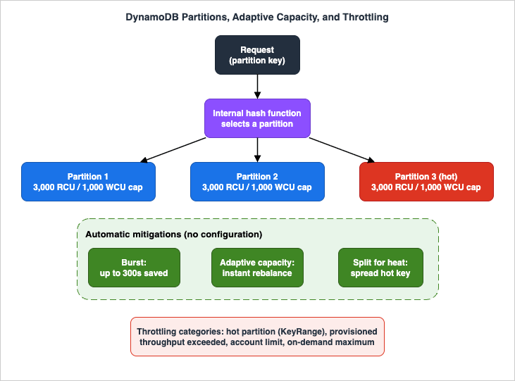
5.2 The hard per-partition limit
Every partition has a fixed ceiling: a single partition can serve at most 3,000 RCUs and 1,000 WCUs, independently for reads and writes. This is the limit that produces table-looks-fine-but-still-throttles symptoms. If your traffic concentrates on one partition key (a "hot" key), that traffic is capped at the partition's 3,000/1,000, no matter how much table-level capacity is provisioned or how high on-demand could scale. A single, consistently hot item can be isolated by DynamoDB onto a partition by itself and served up to that same 3,000 RCU / 1,000 WCU ceiling — but not beyond.5.3 Burst and adaptive capacity
DynamoDB has two automatic mechanisms that absorb imbalance before it becomes throttling:- Burst capacity. When you are not fully using your throughput, DynamoDB reserves a portion of the unused capacity — currently up to five minutes (300 seconds) of it — for later spikes. A short burst can consume these saved units faster than the per-second rate you provisioned. Burst is also drawn on for background tasks without notice. Burst cushions table-level spikes, but partition-level limits are always enforced: burst does not let a single partition exceed 3,000/1,000.
- Adaptive capacity. DynamoDB automatically and instantly boosts throughput for partitions receiving disproportionate traffic, as long as the table's total capacity (and the per-partition maximum) is not exceeded. Adaptive capacity is on by default for every table and GSI, at no cost, and has been instantaneous since 2019 (it formerly took 5–30 minutes). It also isolates frequently accessed items by rebalancing partitions so that hot items do not share a partition — reducing the chance that one hot item starves its neighbors.
There is an important interaction with local secondary indexes: adaptive capacity will not split an item collection across partitions when the table has an LSI. Because LSI data must live in the same partition as the base item it indexes, an item collection with an LSI is pinned to one partition and therefore to that partition's 3,000/1,000 ceiling. This is a concrete operational reason to prefer a GSI over an LSI even when their keys would be identical — the GSI keeps the collection splittable.
5.4 Split for heat — and where it fails
When traffic is uneven across partitions, DynamoDB can apply split for heat: it splits a hot partition so that items sharing a partition key value spread across multiple partitions, lifting the effective throughput for that key above a single partition's limit. Split for heat works on both base tables and GSIs, and it happens silently over several minutes — there is no event; performance simply improves.But split for heat has a sharp edge that explains a recurring production failure: it cannot help an item collection whose sort key only ever increases (a timestamp, a monotonically growing sequence). No matter where DynamoDB cuts the partition, every new write for that partition key lands on the newest (second) partition, so writes for that key remain capped at 1,000 WCU. The same is true for a GSI with a low-cardinality partition key and an ever-increasing sort key. This is why append-only, timestamp-keyed designs throttle on write under load even though the table is healthy — and the fix is a key-design change (write sharding, time bucketing), which the Key Design and GSI/LSI Dictionary covers in detail. Operationally, the takeaway is that not every hot-partition problem can be solved by throwing capacity at it; some require redesigning the key.
5.5 GSI write back pressure
Writes to a base table item that is projected into a GSI must also be written to the index. If the GSI cannot keep up — because its own provisioned capacity is too low, or because the GSI itself has a hot partition that split for heat cannot relieve — the index applies back pressure that throttles writes on the base table. A symptom of "the table is throttling writes" can therefore have its root cause in an under-provisioned or badly-keyed GSI. Always check GSI capacity and GSI throttle metrics when base-table writes throttle unexpectedly.5.6 The four throttling categories
DynamoDB throttles for two reasons — protecting service performance and enforcing cost/quota limits — and the documentation organizes every throttle into four categories (with specific reason codes spanning table/index and read/write):- Key range throughput exceeded (both modes). Consumption to specific partitions exceeds internal partition-level limits — the hot-partition case. Reasons such as
TableWriteKeyRangeThroughputExceededandIndexReadKeyRangeThroughputExceeded. The classic single-item or single-key hot spot lives here. - Provisioned throughput exceeded (provisioned mode). Consumption exceeds the configured RCUs/WCUs for a table or GSI. This is the familiar
ProvisionedThroughputExceededException. Remedy: raise capacity, fix auto scaling targets/maximums, or move to on-demand. - Account-level service quotas exceeded (on-demand mode). A table or GSI exceeds the per-table account-level throughput quota for the Region (40,000 read/write units by default). These quotas are backstops and can be raised via Service Quotas.
- On-demand maximum throughput exceeded (on-demand mode). Consumption exceeds a maximum throughput you configured on the table or GSI (Section 2.2). This is self-inflicted by design — raise or remove the cap if the peak is legitimate.
Knowing which category you are in is the entire diagnosis. The next section is how you tell them apart.
6. Observability and Diagnostics
When DynamoDB throttles, it returns an exception that names the resource and the reason, and each reason maps to specific CloudWatch metrics. Effective diagnosis means reading both the exception and the right metric — not just looking at table-level consumed capacity, which routinely hides partition-level problems.6.1 The metrics that matter
Start with the throttle metrics, but understand their granularity:ThrottledRequestsis incremented once per request when any event in that request is throttled — even if multiple events (the base table write plus several GSI writes) are throttled within it. It is a good "is anything wrong" signal but it understates the extent of throttling, so never size remediation from it alone.ReadThrottleEvents/WriteThrottleEventscount events that exceeded provisioned RCU/WCU on a table or GSI — finer-grained thanThrottledRequests.- Cause-specific event metrics let you pin the category precisely:
ReadKeyRangeThroughputThrottleEvents/WriteKeyRangeThroughputThrottleEvents(partition-level — the hot-partition tell),ReadAccountLimitThrottleEvents/WriteAccountLimitThrottleEvents(account quota), andReadMaxOnDemandThroughputThrottleEvents/WriteMaxOnDemandThroughputThrottleEvents(your configured on-demand cap).
Then read consumption against provision:
ConsumedReadCapacityUnits/ConsumedWriteCapacityUnitsversusProvisionedReadCapacityUnits/ProvisionedWriteCapacityUnitsshow how close you run to the ceiling. For a GSI you must specify bothTableNameandGlobalSecondaryIndexNamedimensions to see index figures.OnlineIndexConsumedWriteCapacitytracks the write capacity consumed by backfilling a newly added GSI — separate from, and additional to, normalConsumedWriteCapacityUnits. Adding a GSI to a busy table without budgeting for this is a common self-inflicted throttle.
The decisive diagnostic move: if
ThrottledRequests is non-zero but ConsumedCapacity sits well below ProvisionedCapacity (or far below what on-demand should serve), you are almost certainly in key range (hot partition) throttling — confirm with WriteKeyRangeThroughputThrottleEvents — and capacity alone will not fix it.# Are partition-level (hot-partition) writes being throttled on a table?
aws cloudwatch get-metric-statistics \
--namespace AWS/DynamoDB \
--metric-name WriteThrottleEvents \
--dimensions Name=TableName,Value=Orders \
--start-time 2026-06-17T00:00:00Z \
--end-time 2026-06-17T01:00:00Z \
--period 60 --statistics Sum6.2 Finding the hot key with Contributor Insights
Metrics tell you that a partition is hot; they do not tell you which key. Amazon CloudWatch Contributor Insights for DynamoDB does. Enabled per table or per GSI, it surfaces the most frequently accessed and most throttled keys at a glance — turning "a partition is hot" into "this specific partition key (or key range) is the problem," which is what you need to drive a key-design fix. CloudWatch charges apply when it is enabled. In a global table, Contributor Insights enablement is not synchronized across replicas and reports only for the Region where the operation occurred, so enable it in each Region you want to analyze.aws dynamodb update-contributor-insights \
--table-name Orders \
--contributor-insights-action ENABLE6.3 A diagnostic workflow
Put together, throttling triage is a short decision sequence:- Read the exception's reason and map it to one of the four categories (Section 5.6).
- Provisioned exceeded → compare
ConsumedvsProvisioned; raise capacity or fix the auto scaling target/maximum, or move to on-demand. - Account limit / on-demand maximum → check the corresponding
*AccountLimit*/*MaxOnDemand*event metrics; request a quota increase or raise/remove the configured maximum. - Key range (hot partition) → confirm with
*KeyRangeThroughput*metrics, identify the offending key with Contributor Insights, and remediate with key design (sharding, time bucketing) — or, for a planned spike that adaptive capacity can satisfy, pre-warm. If a GSI is implicated, check its capacity and watch for base-table back pressure (Section 5.5).
7. Global Tables: Multi-Region, Multi-Active
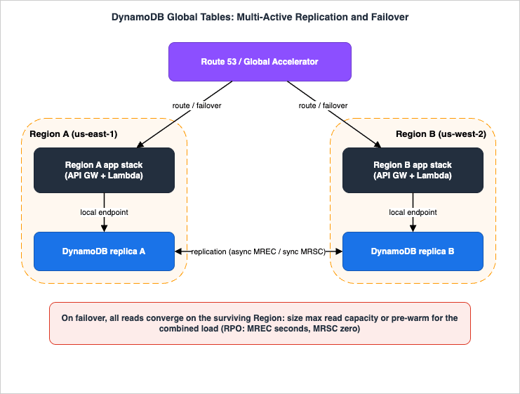
Global tables extend a DynamoDB table across AWS Regions as a multi-active database: every replica accepts both reads and writes, and DynamoDB replicates each write to the other replicas automatically. There are no application changes — replicas share the same table name, key schema, and item data, and you use the same DynamoDB APIs. A single-Region table is designed for 99.99% availability; a global table is designed for 99.999%. The current version is 2019.11.21; always use it rather than the 2017.11.29 legacy version.One architectural fact shapes everything: DynamoDB has no global endpoint. Every request goes to a Regional endpoint and hits the replica local to that Region. The best practice is that an application homed in a Region talks only to its local DynamoDB endpoint; if a Region is impaired, you route end-user traffic to a different Region's full application stack, which talks to its local endpoint — you do not have one Region's compute reach across to another Region's DynamoDB. This is why resilient multi-Region design replicates the compute layer as well as the data layer; global tables give every Regional stack a local copy of the same data. (For the underlying quorum-and-replication model that DynamoDB and other AWS databases use, see the Comparison of AWS Databases Using the Quorum Model.)
The behavior that you must choose deliberately is the consistency mode, set at creation and immutable thereafter, and identical for all replicas. There are two.
The figure shows a multi-active global table, its replication, and a Region failover.
7.1 Multi-Region eventual consistency (MREC)
MREC is the default. Writes are replicated asynchronously, typically within a second, and each replica accepts writes independently. Because two Regions can modify the same item nearly simultaneously, MREC resolves conflicts with last-writer-wins: each item carries a private last-write timestamp, and replication is applied as a conditional write that only takes effect if the incoming timestamp is newer, so all replicas converge on the latest write per item. Conflicts are not recorded in CloudWatch or CloudTrail.The consistency nuance that surprises people: a strongly consistent read against an MREC replica returns the latest version only if the item was last updated in the Region where you read it. If the item was last written in another Region and has not yet replicated, even a strongly consistent read can return stale data. MREC's Recovery Point Objective (RPO) equals the replication lag — usually a few seconds — meaning a Region loss can lose the last few seconds of writes that had not yet replicated. MREC replicas can live in any Region where DynamoDB is available, in any number within the AWS partition, and in same-account or multi-account configurations. You can add or remove a replica (even the original) at any time with no performance impact; DynamoDB handles the initial sync.
7.2 Multi-Region strong consistency (MRSC)
MRSC, generally available since June 30, 2025 (previewed at re:Invent 2024), is for applications that cannot tolerate any stale read or any lost write across Regions — payments, financial ledgers, inventory, critical user-profile state. Its defining behavior: a write is synchronously replicated to at least one other Region before it returns success, and strongly consistent reads on any replica always return the latest item. This delivers an RPO of zero: even a full Region loss cannot lose an acknowledged write.MRSC has a specific shape you must design around:
- It must be deployed in exactly three Regions, as either three full replicas or two replicas plus one witness. A witness stores replicated change data to support the availability/quorum architecture but accepts no reads or writes, lives in a third Region, and incurs no storage or write cost. You choose the Regions (and whether a Region is a replica or the witness) at creation.
- Regions must come from a single Region set: US (N. Virginia, Ohio, Oregon), EU (Ireland, London, Paris, Frankfurt), or AP (Tokyo, Seoul, Osaka). An MRSC table cannot span Region sets.
- You create it from an empty table, and it is same-account only. You cannot add replicas to an existing MRSC table later, and you cannot remove a single replica or witness (you can collapse it back to a single-Region table by removing two).
- Concurrent cross-Region modification of the same item fails the later write with a retryable
ReplicatedWriteConflictException— retry once the other Region's modification settles. - MRSC does not support TTL, local secondary indexes, or the transaction APIs, and eventually consistent reads on MRSC may omit very recent changes (even same-Region ones). Contributor Insights reports per-Region only.
The cost of zero-RPO strong consistency is latency: writes and strongly consistent reads incur cross-Region round trips, so they are slower than MREC's local-latency writes; eventually consistent reads on MRSC have no added latency.
7.3 Choosing a mode
The decision is one question: does the application prioritize low-latency writes and local strong reads (MREC), or global strong consistency with zero RPO (MRSC)? Choose MREC when you can tolerate occasional stale strong reads of cross-Region updates, want the lowest write latency, and can accept an RPO of a few seconds. Choose MRSC when you need strongly consistent reads across Regions, require RPO = 0, and can accept higher write/strong-read latency and the three-Region/same-account/no-TTL-LSI-transactions constraints. Most workloads are well served by MREC; MRSC is the tool for the small set of applications where a lost or stale write is unacceptable.8. Capacity Planning for Global Tables
Multi-Region changes capacity planning in two ways that single-Region thinking misses: replication itself consumes capacity, and a failover concentrates traffic.8.1 Replication consumes write capacity
Every replicated write is a real write in the receiving Region. In provisioned mode, a replica can throttle if the sum of local application writes and inbound replication writes exceeds its provisioned WCU. AWS enforces this by requiring that a global table be either in on-demand mode or in provisioned mode with auto scaling enabled — bare provisioned mode is not allowed for global tables, precisely because replication load is hard to pin to a fixed number. TTL adds a subtlety: a TTL delete is free on the Region that performs it, but it replicates to the other Regions as a delete that does consume replicated write capacity there, so size write capacity (or the on-demand maximum) to cover application writes plus TTL-driven replicated deletes.8.2 The failover convergence problem
The capacity mistake that bites hardest is sizing each Region for its normal share of reads. The whole point of a multi-Region design is that when one Region fails, its traffic moves elsewhere — so a surviving Region may suddenly have to serve all reads. If it was provisioned only for its own slice, it throttles exactly when you need it most.The remedies are explicit in AWS guidance:
- For provisioned global tables, set the maximum read capacity of each Region high enough to absorb the read load of every Region if it all routed there during failover. Read capacity settings are allowed to differ per Region (read patterns differ), so this is a per-Region maximum you must set deliberately.
- For on-demand global tables, there is no provisioned maximum, but the table-level maximum read throughput limit plays the same role — set it high enough for the single-Region-absorbs-everything case.
- For a Region that normally serves little or no read traffic but must absorb a flood on failover, pre-warm its read capacity (Section 4) so it can accept the surge instantly rather than ramping under pressure.
- Use Application Recovery Controller (ARC) readiness checks to confirm that all Regions have comparable table settings and account quotas — a quota mismatch discovered during a failover is a self-inflicted outage.
8.3 What synchronizes across replicas, and what does not
Global tables synchronize some settings automatically and leave others independent. Knowing the taxonomy prevents surprises:- Always synchronized: capacity mode; table and GSI provisioned write capacity and write auto scaling; key schema and GSI definitions; server-side encryption type; TTL; warm throughput; on-demand maximum write throughput; streams definition (in MREC). For provisioned tables, write auto scaling settings (min/max/target) are replicated — though the actual provisioned write capacity floats independently per Region according to each Region's consumption.
- Synchronized but per-replica overridable: table and GSI provisioned read capacity and read auto scaling; table class; on-demand maximum read throughput. This is what lets each Region carry different read capacity. (Note an overridable read setting reverts to the propagated value if the same setting is later changed on any replica.)
- Never synchronized: deletion protection; point-in-time recovery; tags; CloudWatch Contributor Insights enablement; Kinesis Data Streams settings; resource-based policies; streams definition in MRSC mode.
Two operational corollaries: enable PITR, deletion protection, and Contributor Insights in every Region because they do not propagate; and remember that writes to a replica bypass DAX, so DAX caches can serve stale data after a cross-Region write — account for it in read-after-write expectations.
9. End-to-End Architecture Walkthrough
Tie the layers together with a realistic active-active design: a customer-facing application running in two AWS Regions, each with its own full stack (Amazon Route 53 or AWS Global Accelerator in front; Amazon API Gateway and AWS Lambda or containers as the compute layer; a DynamoDB global table as the data layer), built to survive the loss of an entire Region. The data layer is the global table in the figure in Section 7; this section traces a request through it and through a failover.9.1 The normal path
An end user is routed to the nearest healthy Region — by Route 53 latency-based routing, by Global Accelerator's anycast edge, or by client-side logic that picks an endpoint. That Region's compute layer handles the request and talks only to its local DynamoDB endpoint; it never reaches across to the other Region's database. A write lands on the local replica and, under MREC, replicates asynchronously to the other Region within about a second; under MRSC, it is synchronously acknowledged by at least one other Region before returning. Each Region's stack sees the same data because the global table keeps the replicas in sync.9.2 Write models
How the application treats writes across Regions is a deliberate choice with three common shapes:- Write to any Region. Any Region accepts any write; conflicts are resolved by last-writer-wins (MREC) or prevented by synchronous consistency (MRSC). Simplest for the client; appropriate when occasional last-writer-wins resolution is acceptable, or when MRSC guarantees correctness.
- Write to one Region. A single active Region accepts writes at a time; other Regions read locally and forward writes to the active Region. Requires a mechanism — a global coordinator such as ARC routing controls, or application logic — to track which Region is active. Avoids write conflicts entirely.
- Write to your Region. Each data set (for example, each user account) is homed to a Region; the client is directed to that Region. A login service hands back short-lived credentials and the correct Regional endpoint, which also provides a natural moment to re-home a user to a new Region.
Request routing follows from the write model: client-driven routing for write-to-any, compute-layer or coordinator-based routing for write-to-one, and login-directed routing for write-to-your-Region.
9.3 The failover
Suppose the active Region degrades — whether DynamoDB itself or, more commonly, something else in the stack. You do not point the surviving Region's compute at the failed Region's database; you route end-user traffic to the surviving Region's full stack, which serves from its local replica. Two things must already be true for this to work:- The data is there. Under MREC, any writes not yet replicated at the moment of failure are lost (RPO = replication lag); under MRSC, nothing acknowledged is lost (RPO = 0). The consistency mode you chose in Section 7 is your data-loss budget for this moment.
- The capacity is there. All read traffic now converges on one Region. If you sized that Region only for its normal share, it throttles. This is the Section 8.2 convergence problem made concrete: the surviving Region's maximum read capacity — or its pre-warmed read floor — must cover the combined read load, and ARC readiness checks should have confirmed the Regions' settings and quotas match before the incident.
The architecture is only as resilient as its weakest of these two. A global table with perfect replication but a half-sized failover Region is not highly available; neither is a perfectly sized failover Region running MREC for a workload that cannot afford to lose seconds of writes. Capacity planning and consistency-mode choice are the two halves of multi-Region readiness, and both must be decided before, not during, an incident. For broader multi-Region and disaster-recovery patterns beyond DynamoDB, this pairs with high-availability designs for relational stores — see the forthcoming Amazon RDS and Aurora High Availability Guide.
10. Common Pitfalls
- Provisioning for the average and trusting auto scaling for spikes. Auto scaling reacts over minutes; a vertical step throttles before it catches up. Use scheduled scaling, pre-warming, or on-demand for known step-changes, and keep the minimum capacity above zero.
- Leaving a hot partition to "more capacity." If
ThrottledRequestsis non-zero while consumed capacity sits below provisioned, it is partition-level throttling. Adding table capacity does nothing; identify the key with Contributor Insights and fix the key design. - Append-only timestamp keys. A monotonically increasing sort key defeats split for heat and caps the partition key at 1,000 WCU on writes. This is a design fix (write sharding / time bucketing), not a capacity fix — see the Key Design and GSI/LSI Dictionary.
- Under-provisioned or badly-keyed GSIs. A GSI that cannot keep up applies back pressure that throttles base-table writes. Scale and key GSIs as carefully as base tables, and budget
OnlineIndexConsumedWriteCapacitywhen adding one to a busy table. - Choosing LSI when a GSI would do. An LSI pins an item collection to one partition (no split for heat), capping it at per-partition limits. Prefer a GSI unless you specifically need the LSI's strongly consistent local reads.
- Toggling capacity mode reactively. Only four provisioned→on-demand switches are allowed per 24-hour rolling window; automation that flips modes per spike can run out exactly when it needs one more. And switching to on-demand via the console silently deletes auto scaling settings — use the CLI/SDK to preserve them.
- Global table capacity asymmetry. Sizing each Region for its normal read share means a failover overloads the survivor. Size maximum read capacity (or pre-warm) for the single-Region-absorbs-everything case, and validate with ARC readiness checks.
- Designing for MRSC without its constraints. MRSC needs exactly three Regions in one Region set, same-account, an empty starting table, no TTL/LSI/transactions, and tolerance for higher write latency. Discover these at design time, not after you have built on TTL.
- Forgetting that some settings do not replicate. PITR, deletion protection, and Contributor Insights are per-replica — enable them in every Region. And replicated writes bypass DAX, so a cross-Region write can leave a stale DAX cache.
11. Frequently Asked Questions
Q. On-demand or provisioned — which should I choose?A. Default to on-demand: it is the recommended mode, removes capacity planning, and absorbs spikes up to double the previous peak automatically. Choose provisioned (always with auto scaling) only for steady, predictable traffic where you can forecast demand and want a firm rate ceiling. Decide on traffic predictability, operational model, and spike tolerance — not on price (confirm cost on the official pricing page).
Q. Why am I being throttled when I'm under my table's capacity?
A. Almost certainly a hot partition. Every partition caps at 3,000 RCU / 1,000 WCU regardless of table-level capacity, so traffic concentrated on one partition key throttles while the table looks idle. Confirm with the
*KeyRangeThroughput* throttle metrics, find the key with CloudWatch Contributor Insights, and fix it with key design (sharding, time bucketing). If a monotonically increasing sort key is involved, split for heat cannot help — that is a redesign.Q. What does warm throughput actually do?
A. It is the read/write rate your table can serve instantly. The default values are free and reflect historical scaling; pre-warming proactively raises that instantaneous floor for a planned 10x–100x event, without changing billing mode or throughput, asynchronously and non-disruptively. It is a guaranteed minimum (DynamoDB still scales beyond it), it applies to both modes and to all replicas of a global table, and once raised it cannot be lowered.
Q. How do global tables handle a Region failure?
A. Each Region runs a full application stack against its local replica. On failure you route end-user traffic to a surviving Region's stack, which serves from its local replica. Your data-loss exposure is your consistency mode: MREC loses up to the replication lag (RPO = seconds), MRSC loses nothing (RPO = 0). The catch is capacity — all reads may converge on one Region, so its maximum read capacity (or pre-warmed read floor) must cover the combined load, validated ahead of time with ARC readiness checks.
Q. Can I change a global table's consistency mode later?
A. No. The consistency mode (MREC or MRSC) is chosen at creation and is immutable, and all replicas share it. MRSC additionally requires creating from an empty table in exactly three Regions of one Region set, same-account, and you cannot add replicas afterward. Plan the mode before you build.
Q. Does replication consume capacity I need to plan for?
A. Yes. Each replicated write is a real write in the receiving Region, so for provisioned global tables a replica throttles if local writes plus inbound replication exceed its WCU — which is why global tables must be on-demand or provisioned-with-auto-scaling. TTL deletes are free where they run but replicate as capacity-consuming deletes elsewhere, so size write capacity (or the on-demand maximum) for writes plus replicated TTL deletes.
12. Summary
DynamoDB capacity is four layers that you operate together. The mode (on-demand by default; provisioned with auto scaling for steady traffic) sets how capacity is managed. The elasticity features — auto scaling's reactive control loop, on-demand's double-the-peak scaling, and warm throughput's instantaneous, pre-warmable floor — decide how fast and how much the table can absorb. The partition layer, with its hard 3,000 RCU / 1,000 WCU per-partition limits, burst, instant adaptive capacity, and split for heat, is where most real throttling happens and where capacity alone sometimes cannot help. And observability — the four throttle categories, the cause-specific metrics, and Contributor Insights for hot keys — is how you tell those cases apart.Multi-Region adds global tables, where the consistency-mode choice (MREC's low-latency, last-writer-wins, seconds-of-RPO model versus MRSC's synchronous, zero-RPO, three-Region model) is a data-loss decision, and where capacity planning must assume failover convergence — one Region absorbing everyone's reads. Get the mode, the elasticity, the keys, and the multi-Region capacity right, and a well-designed table stays a well-running one.
For the design half of DynamoDB — partition keys, secondary indexes, single-table modeling, and the key-design remedies for hot partitions referenced throughout — continue with the Key Design and GSI/LSI Dictionary and the Single Table Design Guide; for terminology and history, the AWS Database Glossary and the Amazon DynamoDB timeline; and for the replication model behind global tables, the Comparison of AWS Databases Using the Quorum Model.
13. References
- DynamoDB throughput capacity (capacity modes) - Amazon DynamoDB Developer Guide
- DynamoDB on-demand capacity mode - Amazon DynamoDB Developer Guide
- Considerations when switching capacity modes in DynamoDB - Amazon DynamoDB Developer Guide
- Managing throughput capacity automatically with DynamoDB auto scaling - Amazon DynamoDB Developer Guide
- Understanding DynamoDB warm throughput - Amazon DynamoDB Developer Guide
- DynamoDB burst and adaptive capacity - Amazon DynamoDB Developer Guide
- Partitions and data distribution in DynamoDB - Amazon DynamoDB Developer Guide
- Troubleshooting throttling in Amazon DynamoDB - Amazon DynamoDB Developer Guide
- CloudWatch throttling metrics - Amazon DynamoDB Developer Guide
- Analyzing data access using CloudWatch Contributor Insights for DynamoDB - Amazon DynamoDB Developer Guide
- How DynamoDB global tables work (consistency modes) - Amazon DynamoDB Developer Guide
- Using DynamoDB global tables (design best practices) - Amazon DynamoDB Developer Guide
- Throughput capacity planning for DynamoDB global tables - Amazon DynamoDB Developer Guide
- Quotas in Amazon DynamoDB - Amazon DynamoDB Developer Guide
- Build the highest resilience apps with multi-Region strong consistency in Amazon DynamoDB global tables - AWS News Blog
- Pre-warming Amazon DynamoDB tables with warm throughput - AWS Database Blog
- Scaling DynamoDB: How partitions, hot keys, and split for heat impact performance - AWS Database Blog
- Amazon DynamoDB pricing
Related Articles
- Amazon DynamoDB Key Design and GSI/LSI Dictionary — the design companion: partition/sort key choices, GSI vs LSI, and the key-design remedies for hot partitions (write/read sharding, time bucketing) delegated throughout this guide.
- Amazon DynamoDB Single Table Design Guide — modeling many entities and access patterns in one table.
- AWS History and Timeline regarding Amazon DynamoDB — when on-demand, adaptive capacity, global tables, warm throughput, and MRSC each shipped.
- Comparison of AWS Databases Using the Quorum Model — the replication and quorum model behind global tables and strong consistency.
- AWS Database Glossary — definitions for the capacity, partition, and replication terms used here.
- Amazon RDS and Aurora High Availability Guide — the relational counterpart to this guide's multi-Region resilience patterns.
References:
Tech Blog with curated related content
Written by Hidekazu Konishi