DynamoDB Key Design Dictionary: PK/SK, GSI/LSI Selection, Hot Partition Avoidance, and Re-Keying Patterns

First Published: 2026-05-08
Last Updated: 2026-05-08

This article is a lookup dictionary for DynamoDB key design. Each section answers a concrete question — "I have this access pattern, how do I lay out PK/SK?", "GSI or LSI for this case?", "How do I split a hot partition?", "How do I re-key a live table without downtime?" — and gives you the smallest correct answer with a worked example.

Where the companion article Amazon DynamoDB Single Table Design Complete Guide explains the philosophy of access-pattern-driven modeling with five canonical patterns, this dictionary catalogs PK/SK patterns by use case across five categories, plus GSI vs LSI selection criteria, hot-partition avoidance, online re-keying procedures, and an anti-pattern catalog. Read that one first if you have not internalized the access-pattern-first methodology; come here when you have a specific design decision to make and want a quick, opinionated answer.

Note: Service quotas (GSI count, item collection size, per-partition throughput) are stated as defaults at the time of writing. AWS occasionally raises soft limits and adds new defaults; for production capacity planning always confirm the current values on the DynamoDB Service Quotas page.

0. How to Use This Dictionary

This article is organized so you can jump to the section that answers your current question:

Section 1: DynamoDB Data Model in 60 Seconds — minimum vocabulary you need to follow the rest of the dictionary.
Section 2: Partition Key vs Sort Key — Design Decisions — when to use a simple PK only, when to use a composite PK+SK, how to structure the SK.
Section 3: GSI vs LSI Decision Matrix — the single most asked question, answered with a one-page decision flow and a comparison table.
Section 4: Key Design Patterns by Use Case — the core catalog. Find your access pattern, copy the PK/SK structure, adapt the boto3 sample.
Section 5: Hot Partition Avoidance Techniques — when adaptive capacity is not enough.
Section 6: Migration and Re-Keying Strategies — change the keys of a live table without downtime.
Section 7: Anti-Patterns Catalog — the design choices that look right and fail in production.
Section 8: Summary and Section 9: References.

Throughout, code examples use Python with boto3 against DynamoDB tables that follow the conventional generic-attribute schema (PK, SK, GSI1PK, GSI1SK, ...). Translate freely to your SDK of choice — the design decisions are language-independent.

1. DynamoDB Data Model in 60 Seconds

This section is deliberately minimal. If any term below is unfamiliar, read the Single Table Design Complete Guide before continuing.

Item: a row. Up to 400 KB including attribute names and values.
Partition Key (PK): the hash that determines which physical partition holds the item. Required. Picking it well is the single most consequential decision in DynamoDB.
Sort Key (SK): optional second attribute. When present, items with the same PK are stored together, sorted by SK byte order. Together (PK, SK) form the primary key.
Item Collection: the set of all items with the same PK value. Maximum 10 GB only when the table has at least one Local Secondary Index; without LSIs, item collections can grow without that ceiling.
Global Secondary Index (GSI): a separate physical structure with its own PK/SK. Asynchronously maintained. Eventually consistent. Default soft limit of 20 per table (raise via the AWS Service Quotas console).
Local Secondary Index (LSI): an alternate sort order on the same partition as the base table. Synchronously maintained. Strongly consistent on demand. Up to 5 per table, created at table creation only, never added or removed afterward.
DynamoDB Streams: a 24-hour change-data-capture log per table, consumed natively by Lambda Event Source Mappings and Kinesis Client Library applications. A separate opt-in feature, Kinesis Data Streams for DynamoDB, exports the same change records to a Kinesis Data Stream that you own (longer retention, fan-out, multi-region pipelines). Both are the backbone of online migrations and asynchronous aggregation.

The canonical operations against this model are GetItem (single primary-key lookup), Query (scan within one PK, optionally bounded by SK conditions), and BatchGetItem / BatchWriteItem (parallel multi-key fetch / write, up to 100 / 25 items respectively). Scan is for one-off admin work; treat its appearance in production code as a bug.

For a comparison of how DynamoDB's quorum model relates to other AWS databases (Aurora, Neptune, OpenSearch), see the companion article Summary of Differences and Commonalities in AWS Database Services using the Quorum Model.

2. Partition Key vs Sort Key — Design Decisions

2.1 PK Alone vs Composite (PK + SK)

Use a simple PK (no SK) only for tables that store a single item per logical entity with no need to fetch siblings together. Examples that fit:

Token vaults (PK = jti, item = JWT metadata + revocation flag).
Distributed lock manager (PK = lock_name, item = lease holder + expiry).
Simple session stores (PK = session_id, item = user identity + expiry).

Everything else — users, orders, devices, documents, anything that has children or versions — should use a composite PK + SK from the very first design pass. Adding a sort key later requires a full re-keying migration (Section 6). Adding it on day one costs you nothing.

The default schema for any non-trivial table:

PK = ENTITY#<entity_id>
SK = METADATA               (or #META, or "v0_<entity>")

The literal METADATA (or any fixed sentinel) is a placeholder so future child items can join the same item collection without colliding with the parent. This pattern is sometimes called the "reserved root".

2.2 Sort Key Structure — Hierarchical, Composite, Sortable

The sort key is your secondary access path within a partition. Three structural choices dominate, and you will use all three across a real table.

Hierarchical SK — encodes a fixed hierarchy from coarse to fine:

SK = <Continent>#<Country>#<State>#<City>#<ZipCode>

A begins_with("ASIA#JAPAN#") query returns all Japan locations; begins_with("ASIA#JAPAN#TOKYO#") narrows to Tokyo. The order of segments is locked at design time — any later change to the hierarchy means a full re-key.

Composite filter SK — encodes multiple filter dimensions in fixed order:

SK = REGION#<region>#STATUS#<status>#DATE#<YYYY-MM-DD>#ORDER#<order_id>

You can filter by leading prefix (region, then status, then date), but you cannot filter by a non-leading dimension without a separate GSI. If you need "all orders on a date across all regions", it requires either a Filter Expression (which still consumes RCU for the whole scanned range) or a GSI keyed by date.

Sortable timestamp SK — encodes time directly so chronological ordering is free:

SK = EVENT#<ISO8601_timestamp>#<event_id>
SK = EVENT#<ULID>           # ULID/KSUID encodes a millisecond timestamp in its leading bits

Use ULID/KSUID rather than UUIDv4 when you want the SK itself to encode time without a separate timestamp attribute. UUIDv7 is functionally equivalent for this purpose.

One rule that catches more bugs than any other: prefix every SK segment with a type tag (USER#, ORDER#, EVENT#). It costs a few bytes and lets begins_with queries cleanly target one entity type out of an overloaded item collection. The cost of forgetting the prefix is debuggability — Query(PK=...) returns an undifferentiated stream of items and you cannot tell types apart at 3 AM.

2.3 Generic Key Names + Type Attribute

Single-table designs that mix multiple entity types in one table use generic key names rather than entity-specific ones:

Bad:   userId (PK), addressId (SK)
Good:  PK, SK, with a separate Type attribute on each item

Generic names let the same column hold USER#u_123 on a User item and ORDER#o_456 on an Order item without semantic confusion. The Type attribute (Type = "User", Type = "Order", Type = "Address") is essential for stream-processing Lambdas that need to route updates to type-specific handlers, and for ad-hoc CLI debugging.

GSIs follow the same convention with GSI1PK, GSI1SK, GSI2PK, GSI2SK, etc. — generic names so a single GSI can be overloaded for multiple access patterns (Section 3.3).

3. GSI vs LSI Decision Matrix

This is the most-asked DynamoDB design question. The answer fits on one page.

3.1 The Comparison Table

The official Secondary Indexes page in the Developer Guide is the source of record. The decision-relevant differences:
* You can sort the table by clicking on the column name.

Characteristic	Global Secondary Index (GSI)	Local Secondary Index (LSI)
Partition key relationship	Any attribute. PK can differ from base table.	Must share the base table's PK. Only SK differs.
Item collection size limit	None	10 GB per PK value (cap applies to the base table once any LSI is defined)
Add or remove after table creation	Yes — online operation	No — created at table creation only, cannot delete
Query scope	Whole table, scattered across all partitions	Single partition (one PK value)
Read consistency	Eventual only	Eventual or strong (caller chooses)
Provisioned throughput	Separate from base table	Shares base table's throughput
Non-projected attribute fetch	Not possible	Possible (extra RCU, server-side fetch)
Default count limit per table	20 (soft limit, raise via Service Quotas)	5 (hard limit, not adjustable)

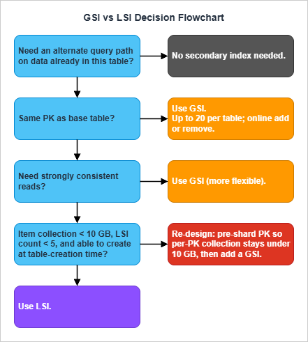
3.2 LSI vs GSI — The Decision in One Sentence Each

Choose an LSI when you need a strongly consistent read on an alternate sort order on data that is already partitioned correctly, and you can guarantee per-PK item collections stay under 10 GB forever.

Choose a GSI in every other case — and as the default when you are uncertain. GSIs are more flexible (any PK), online (add/remove anytime), and unconstrained by the 10 GB ceiling.

The hidden cost of an LSI is the 10 GB ceiling on every item collection in the table that activates the moment any LSI exists. A table that worked fine for years can hit a wall when a single popular PK accumulates enough data to exceed 10 GB; the only fix is a re-keying migration. GSIs do not impose this constraint.

3.3 Sparse, Inverted, and Overloaded Indexes

These three index patterns are not separate index types — they are uses of GSIs that recur often enough to deserve names.

Sparse index — only items that have the indexed attribute appear in the GSI. Items where the GSI key attribute is absent are filtered out automatically. Use when the attribute is present on a minority of items: "all soft-deleted orders", "all users with verified email", "all orders pending review". The GSI cost is proportional to the indexed-item count, not the table size.

Base item (active order):    {PK=ORDER#abc, SK=METADATA, status="ACTIVE"}
Base item (deleted order):   {PK=ORDER#xyz, SK=METADATA, status="DELETED",
                              GSI1PK="DELETED_ORDER", GSI1SK="2026-05-01T..."}

Only the deleted order appears in GSI1.

Inverted index — the GSI swaps PK and SK from the base table. Used to query a many-to-many relationship from either side without duplicating edge data:

Base table: PK=USER#alice,  SK=GROUP#42      (membership edge)
GSI1:       GSI1PK=GROUP#42, GSI1SK=USER#alice
Query the base table for "groups of alice". Query GSI1 for "members of group 42".

Overloaded GSI — a single GSI serves multiple access patterns by storing semantically different values in GSI1PK / GSI1SK depending on the item type. The classic example from AWS documentation: an Employees table where one GSI overloads GSI1PK to hold employee name on Employee items, warehouse ID on Inventory items, hire date on HR records, etc. — all queryable through the same index. See GSI Overloading for the canonical example.

Overloading is what lets a real single-table design ship five access patterns on three GSIs instead of one GSI per pattern. Plan two or three "reserve" GSIs from day one (GSI1, GSI2, GSI3) and treat them as overload slots, not as dedicated single-purpose indexes.

4. Key Design Patterns by Use Case

This is the core of the dictionary. The patterns are grouped into five categories. Each pattern follows the same structure:

Use case — one-line statement of the access pattern.
PK/SK — the key layout, with sentinel values shown literally.
Access patterns — the read/write operations enabled by the layout, with boto3-style pseudocode.
GSI/LSI — when an index is required, the index keys and projection.
Pitfalls — the design choices that look right and fail in production.

The patterns assume Python boto3 Table objects bound to a single-table schema with generic attribute names (PK, SK, GSI1PK, GSI1SK).

4.1 Category 1: Lookup & CRUD

These four patterns cover ~70% of pre-launch CRUD code in a typical service.

Pattern P1: Single-Entity Lookup by ID

Use case: Retrieve one entity (user, product, order, document) by its identifier. The most common access pattern in any service.

PK/SK:

PK = USER#<userId>
SK = METADATA

The SK = METADATA sentinel reserves the partition for child items (profile, addresses, orders) added later under the same user.

Access patterns:

# Single user fetch (O(1))
resp = table.get_item(Key={"PK": "USER#u_001", "SK": "METADATA"})
user = resp.get("Item")

# User plus all child items in one query
resp = table.query(KeyConditionExpression=Key("PK").eq("USER#u_001"))
items = resp["Items"]   # METADATA + child items

Pitfall: Using a bare entity ID (PK = "u_001") as the sole PK with no USER# prefix means you cannot distinguish entity types when mixing them in one table. Always use a type prefix from day one — adding it later is a re-keying migration.

Pattern P2: Composite Uniqueness (Multi-Attribute Unique Constraint)

Use case: Enforce uniqueness across a combination of attributes (e.g., one email per user, one slug per tenant) without a relational unique constraint.

PK/SK:

Primary item:    PK = USER#<userId>,           SK = METADATA
Constraint item: PK = USEREMAIL#<email>,       SK = CONSTRAINT

The two items are written atomically in a TransactWriteItems call with a ConditionExpression that fails if the constraint item already exists.

Access patterns:

# Atomic registration: create user only if email not yet taken
table.meta.client.transact_write_items(
    TransactItems=[
        {
            "Put": {
                "TableName": table.name,
                "Item": {"PK": "USER#u_001", "SK": "METADATA",
                         "email": "alice@example.com", "name": "Alice"},
                "ConditionExpression": "attribute_not_exists(PK)",
            }
        },
        {
            "Put": {
                "TableName": table.name,
                "Item": {"PK": "USEREMAIL#alice@example.com", "SK": "CONSTRAINT",
                         "userId": "u_001"},
                "ConditionExpression": "attribute_not_exists(PK)",
            }
        },
    ]
)

Pitfall: The constraint item must be deleted (in a transaction) when the primary item is deleted. Forgetting this leaves a "zombie constraint" that permanently blocks reuse of the email. Always pair primary delete with constraint delete in TransactWriteItems.

Pattern P3: Lookup by Alternative Key (Sparse GSI)

Use case: Resolve a user by an alternative identifier (email, OAuth provider ID, employee number, external system reference) that not every item necessarily has.

PK/SK:

Base table: PK = USER#<userId>, SK = METADATA
            Attributes set when applicable:
              GSI1PK = EMAIL#<email>
              GSI1SK = USER#<userId>

GSI1: GSI1PK partition key, GSI1SK sort key.
      Sparse — items without GSI1PK are excluded automatically.

Access patterns:

# Resolve email to userId
resp = table.query(
    IndexName="GSI1",
    KeyConditionExpression=Key("GSI1PK").eq("EMAIL#alice@example.com"),
)
user_item = resp["Items"][0] if resp["Items"] else None

The same GSI can be overloaded with GSI1PK = OAUTH#<provider>#<external_id> or GSI1PK = EMPNO#<employee_number> to resolve other alternative keys through the same index.

Pitfall: If the alternative-key attribute ends up on a majority of items, the GSI is no longer sparse and you have paid for a full-size second index without the cost benefit. Sparse GSIs only make economic sense when the attribute is present on a clear minority of items.

Pattern P4: Soft Delete with TTL

Use case: Mark items as logically deleted (for undo, audit, recycling-bin UX) without immediate physical removal. Eventually purged by DynamoDB TTL.

PK/SK:

Active item:   PK=ORDER#<orderId>, SK=METADATA, status="ACTIVE"
Soft-deleted:  PK=ORDER#<orderId>, SK=METADATA, status="DELETED",
               deletedAt=<epoch>, ttl=<epoch + 30d>,
               GSI1PK="DELETED_ORDER", GSI1SK=<ISO deletedAt>

Access patterns:

# Soft delete
table.update_item(
    Key={"PK": "ORDER#o_001", "SK": "METADATA"},
    UpdateExpression=("SET #s = :deleted, deletedAt = :now, "
                      "#ttl = :expiry, GSI1PK = :gpk, GSI1SK = :gsk"),
    ExpressionAttributeNames={"#s": "status", "#ttl": "ttl"},
    ExpressionAttributeValues={
        ":deleted": "DELETED",
        ":now": int(time.time()),
        ":expiry": int(time.time()) + 30 * 86400,
        ":gpk": "DELETED_ORDER",
        ":gsk": datetime.utcnow().isoformat(),
    },
)

# Recently deleted orders, newest first (recycle bin)
resp = table.query(
    IndexName="GSI1",
    KeyConditionExpression=Key("GSI1PK").eq("DELETED_ORDER"),
    ScanIndexForward=False,
    Limit=20,
)

Pitfall: TTL deletion is asynchronous and can lag up to 48 hours. Do not rely on TTL timing for correctness. Always filter active reads on status = "ACTIVE" (or use a sparse GSI for active items) so soft-deleted items are excluded immediately, regardless of when TTL physically removes them.

4.2 Category 2: One-to-Many & Hierarchy

These patterns model parent-child and tree relationships within a partition.

Pattern P5: Parent-Child with Prefix Sort Key

Use case: Store a parent entity and its children together so a single Query returns the complete aggregate (user + profile + addresses + orders).

PK/SK:

PK = USER#<userId>
SK = METADATA              (parent)
SK = PROFILE               (one profile child)
SK = ADDR#<addrId>         (zero-or-more address children)
SK = ORDER#<orderId>       (zero-or-more order children; orderId = ULID for time sort)

Access patterns:

# Whole user aggregate in one Query
resp = table.query(KeyConditionExpression=Key("PK").eq("USER#u_001"))

# Only the addresses
resp = table.query(
    KeyConditionExpression=Key("PK").eq("USER#u_001")
        & Key("SK").begins_with("ADDR#"),
)

# Latest 10 orders (ULID sorts chronologically)
resp = table.query(
    KeyConditionExpression=Key("PK").eq("USER#u_001")
        & Key("SK").begins_with("ORDER#"),
    ScanIndexForward=False, Limit=10,
)

Pitfall: Unbounded children. If a user can have millions of orders, the item collection grows without limit, and read amplification on Query(PK=USER#...) becomes severe even with Limit. For unbounded children, separate them into a different partition with a time-bucketed PK (Pattern P10), or move them entirely to a child table. Also, if any LSI exists on the table, item collections are capped at 10 GB and a popular user could hit the wall.

Pattern P6: Materialized Path Tree

Use case: Hierarchies like organizational trees, file-system paths, category taxonomies, comment threads. Subtree retrieval must be a single Query.

PK/SK:

PK = ORG#<root_id>
SK = PATH#<root>#<level1>#<level2>#<level3>

Concrete example for a four-level org chart:

PK=ORG#acme  SK=PATH#root
PK=ORG#acme  SK=PATH#root#engineering
PK=ORG#acme  SK=PATH#root#engineering#cloud
PK=ORG#acme  SK=PATH#root#engineering#cloud#aws_squad
PK=ORG#acme  SK=PATH#root#sales
PK=ORG#acme  SK=PATH#root#sales#emea

Access patterns:

# Entire engineering subtree
resp = table.query(
    KeyConditionExpression=Key("PK").eq("ORG#acme")
        & Key("SK").begins_with("PATH#root#engineering"),
)

# Direct children of engineering only (post-filter by depth)
direct = [i for i in resp["Items"] if i["SK"].count("#") == 3]

Pitfall: Tree mutations are expensive. Moving a subtree to a different parent requires rewriting the SK on every descendant — there is no atomic "rename path prefix" operation. Plan tree edits as offline jobs. Also, querying upward (ancestors of node X) requires either parsing the path string client-side or maintaining a parent-pointer GSI.

Pattern P7: Adjacency List for Many-to-Many

Use case: Bidirectional graph relationships — users and groups, students and courses, tags and articles, invoices and line items.

PK/SK:

Base table: PK = USER#<userId>,  SK = GROUP#<groupId>   (membership edge, queryable from user side)

GSI1 (inverted):
  GSI1PK = SK value (= GROUP#<groupId>)
  GSI1SK = PK value (= USER#<userId>)

The same item is indexed twice, once in the base table keyed by user and once in GSI1 keyed by group. No edge data is duplicated; only an additional index exists.

Access patterns:

# Groups for a user
resp = table.query(
    KeyConditionExpression=Key("PK").eq("USER#u_001")
        & Key("SK").begins_with("GROUP#"),
)

# Users in a group (via inverted GSI)
resp = table.query(
    IndexName="GSI1",
    KeyConditionExpression=Key("GSI1PK").eq("GROUP#g_42")
        & Key("GSI1SK").begins_with("USER#"),
)

Pitfall: Hot-spot nodes. A single popular group with millions of members puts all those edges on one GSI partition. For high-fan-out nodes, shard the GSI key (GSI1PK = GROUP#g_42#shard#0..N) and scatter-gather reads — the same write-sharding technique covered in Section 5.2. Plan the shard suffix at design time even if you only use a single shard initially; introducing it later is a re-key.

See Best Practices for Managing Many-to-Many Relationships for the canonical AWS treatment.

Pattern P8: Hierarchical Aggregation / Rollup

Use case: Maintain pre-computed aggregates (per-day totals, per-month rollups, leaderboards) updated asynchronously by stream processing.

PK/SK:

Event item: PK = SONG#<songId>, SK = PLAY#<eventId>, playedAt=...

Aggregate item (sparse, only on rollup items):
  PK = SONG#<songId>, SK = AGG#<YYYY-MM>
  Attributes: month=<YYYY-MM>, playCount=<int>
  GSI1PK = MONTH#<YYYY-MM>      (GSI for "top songs in month")
  GSI1SK = playCount             (sort by count)

Access patterns:

# Atomic increment on event arrival (Lambda from DynamoDB Streams).
# DynamoDB rejects an UpdateExpression that names the same attribute in two
# action clauses (e.g., ADD playCount + SET GSI1SK = playCount in one call) with
# "Two document paths overlap with each other", so split the update into two
# steps: increment the counter, then mirror the post-increment value into the
# GSI sort key. ReturnValues="UPDATED_NEW" returns the value after ADD applied.
resp = table.update_item(
    Key={"PK": f"SONG#{song_id}", "SK": f"AGG#{month}"},
    UpdateExpression="ADD playCount :one SET #m = :m, GSI1PK = :gpk",
    ExpressionAttributeNames={"#m": "month"},
    ExpressionAttributeValues={
        ":one": 1, ":m": month, ":gpk": f"MONTH#{month}",
    },
    ReturnValues="UPDATED_NEW",
)
new_count = int(resp["Attributes"]["playCount"])
table.update_item(
    Key={"PK": f"SONG#{song_id}", "SK": f"AGG#{month}"},
    UpdateExpression="SET GSI1SK = :sk",
    ExpressionAttributeValues={":sk": new_count},
)

# Top 10 songs for a month
resp = table.query(
    IndexName="GSI1",
    KeyConditionExpression=Key("GSI1PK").eq("MONTH#2026-05"),
    ScanIndexForward=False, Limit=10,
)

Pitfall: Stream processors are at-least-once; Lambda retries can double-count. Either make the increment idempotent by tracking processed event IDs (e.g., conditional ADD only if eventId not in a deduplication set), or accept the count as approximate. For exact counts (financial, regulatory), use TransactWriteItems to atomically write the event item and increment the aggregate — but be aware this consumes 2× the WCU and limits per-transaction action count to 100. The two-step UpdateItem pattern shown above is also non-atomic across the two calls; in production, mirror GSI1SK from a DynamoDB Streams consumer reading the post-image so retries converge on the same value.

See Best Practices for Managing Aggregations and Sparse GSI Patterns for the official pattern.

4.3 Category 3: Time-Series & Event Stream

These patterns optimize for append-heavy workloads and time-range queries.

Pattern P9: Append-Only Events with KSUID/ULID Sort Key

Use case: Event sourcing, order state machines, chat messages, audit logs — anywhere immutable events accumulate against an aggregate, with strict chronological ordering.

PK/SK:

PK = ORDER#<orderId>
SK = EVENT#<ULID>

ULID and KSUID encode a millisecond timestamp in their leading bits and are designed to sort lexicographically in chronological order. Use the monotonic mode of your ULID library to break ties within the same millisecond, or you risk out-of-order items under high write rates.

Access patterns:

# All events for an order, in order
resp = table.query(
    KeyConditionExpression=Key("PK").eq("ORDER#o_001")
        & Key("SK").begins_with("EVENT#"),
)

# Most recent event only
resp = table.query(
    KeyConditionExpression=Key("PK").eq("ORDER#o_001")
        & Key("SK").begins_with("EVENT#"),
    ScanIndexForward=False, Limit=1,
)

# Events in a time window (ULID time-prefix encoding lets between() bound the range)
start_ulid = ulid_at(start_timestamp)
end_ulid   = ulid_at(end_timestamp)
resp = table.query(
    KeyConditionExpression=Key("PK").eq("ORDER#o_001")
        & Key("SK").between(f"EVENT#{start_ulid}", f"EVENT#{end_ulid}"),
)

Pitfall: Distributed clock skew. ULIDs generated on different hosts at the same wall-clock moment can interleave out of order across hosts. If strict global ordering is required (e.g., financial event sourcing), prefer a centrally generated monotonic sequence (an Aurora SERIAL, a DynamoDB counter, or a managed source like Kinesis) over distributed ULID generation.

Pattern P10: Time-Bucketed Partition Key

Use case: High-volume time series — IoT sensor readings, request logs, security telemetry — where a single device or tenant generates more events than a single partition can hold (10 GB cap with LSIs) or sustain (1,000 WCU/s per partition).

PK/SK:

PK = DEVICE#<deviceId>#<YYYY-MM>     (monthly bucket — adjust granularity as needed)
SK = <ISO8601 timestamp>#<event_id>

For per-device write rates above ~500 WCU/s sustained, drop to daily or hourly buckets:

PK = DEVICE#<deviceId>#<YYYY-MM-DD>
PK = DEVICE#<deviceId>#<YYYY-MM-DDTHH>

Access patterns:

# Readings for a device on a specific day
resp = table.query(
    KeyConditionExpression=Key("PK").eq("DEVICE#d_001#2026-05")
        & Key("SK").begins_with("2026-05-15"),
)

# Multi-month query: parallel queries across N buckets, application-side merge
import asyncio, aioboto3
async def query_window(device_id, months):
    async with aioboto3.Session().resource("dynamodb") as ddb:
        tbl = await ddb.Table("AppTable")
        results = await asyncio.gather(*[
            tbl.query(KeyConditionExpression=Key("PK").eq(f"DEVICE#{device_id}#{m}"))
            for m in months
        ])
    return [item for r in results for item in r["Items"]]

Pitfall: Choosing the bucket too coarse (annual) lets popular devices hit the 10 GB partition wall when LSIs are present. Choosing too fine (hourly) multiplies the read fan-out cost — a 30-day query becomes 720 parallel queries. The right granularity is roughly 1 / (peak_writes_per_second / 500) rounded to a calendar boundary. See Best Practices for Time Series Data for the AWS-recommended approach including the tactic of rolling cold time periods to a smaller capacity tier.

Pattern P11: Latest-N with v0 Sentinel

Use case: Always-current latest value plus full revision history, with O(1) latest read. Equipment audit trails, document revisions, compliance-grade configuration items.

PK/SK:

PK = EQUIPMENT#<id>
SK = v0_AUDIT          (always overwritten with the latest copy)
SK = v1_AUDIT          (immutable historic version 1)
SK = v2_AUDIT          (immutable historic version 2)
SK = vN_AUDIT

The v0_ sentinel sorts before v1_ lexicographically because 0 < 1 in ASCII. GetItem(SK=v0_AUDIT) always returns the latest version in O(1) without a Query.

Zero-padding requirement: Lexicographic sort breaks once you cross a digit boundary — v10_ sorts between v1_ and v2_, not after v9_. Pad the version number to a fixed width that comfortably exceeds the maximum revision count (e.g., v0000_, v0001_, ..., v9999_) so history queries return revisions in the intuitive numeric order. The same padding rule applies to any numeric component you embed in an SK.

Access patterns:

# Latest version, O(1)
resp = table.get_item(Key={"PK": "EQUIPMENT#e_001", "SK": "v0_AUDIT"})
latest = resp.get("Item")

# Full revision history (excludes v0 sentinel)
resp = table.query(
    KeyConditionExpression=Key("PK").eq("EQUIPMENT#e_001")
        & Key("SK").begins_with("v"),
)
history = [i for i in resp["Items"] if i["SK"] != "v0_AUDIT"]

# Update: write new vN AND overwrite v0 atomically
table.meta.client.transact_write_items(TransactItems=[
    {"Put": {"TableName": tbl_name,
             "Item": {"PK": pk, "SK": f"v{new_n}_AUDIT", **new_attrs}}},
    {"Put": {"TableName": tbl_name,
             "Item": {"PK": pk, "SK": "v0_AUDIT", **new_attrs}}},
])

Pitfall: Without the transaction, a partial failure (new vN written, v0 overwrite fails) leaves v0 stale. Always use TransactWriteItems. Also add an optimistic-locking version attribute so concurrent updaters cannot silently overwrite each other's work — the loser gets TransactionCanceledException and retries with the new state.

See Best Practices for Sort Keys — Version Control for the official version-control pattern.

Pattern P12: Inverted GSI for Entity-Time Scan

Use case: Admin and reporting queries like "all users sorted by signup date" or "all orders in the last 24 hours across all customers". A full table scan is unacceptable.

PK/SK:

Base item: PK = USER#<userId>, SK = METADATA
  Attributes: GSI1PK = "USER", GSI1SK = <ISO createdAt>

GSI1: GSI1PK = entity type (constant per type),
      GSI1SK = createdAt (timestamp).

Access patterns:

# Newest 50 users
resp = table.query(
    IndexName="GSI1",
    KeyConditionExpression=Key("GSI1PK").eq("USER"),
    ScanIndexForward=False, Limit=50,
)

# All orders in May 2026
resp = table.query(
    IndexName="GSI1",
    KeyConditionExpression=Key("GSI1PK").eq("ORDER")
        & Key("GSI1SK").between("2026-05-01", "2026-06-01"),
)

Pitfall: A constant GSI1PK = "USER" puts every user item in one GSI partition. At ten million active users this becomes a hot read partition. Add a low-cardinality shard suffix derived from the timestamp itself (GSI1PK = USER#<YYYY-MM>) to spread the load, and accept that range queries now require fan-out across month buckets. If sub-second freshness is required, the inverted-GSI approach is the wrong tool — use a streaming aggregation into OpenSearch or a materialized view in Aurora.

4.4 Category 4: Search-like & Multi-Tenant

These patterns support filtered listings, multi-dimensional filters, and per-tenant isolation.

Pattern P13: Multi-Tenant Prefixed PK

Use case: SaaS pooled-tenancy model. All tenants share one table, isolation is enforced by always prefixing the PK with the tenant identifier.

PK/SK:

PK = TENANT#<tenantId>
SK = USER#<userId>           (or ORDER#<orderId>, CONFIG#<configKey>, ...)

Access patterns:

# All users for a tenant
resp = table.query(
    KeyConditionExpression=Key("PK").eq("TENANT#acme")
        & Key("SK").begins_with("USER#"),
)

IAM enforces tenant isolation via the dynamodb:LeadingKeys condition key, scoped to the caller's tenant ID:

{
  "Effect": "Allow",
  "Action": ["dynamodb:GetItem", "dynamodb:Query", "dynamodb:PutItem"],
  "Resource": "arn:aws:dynamodb:*:*:table/AppTable",
  "Condition": {
    "ForAllValues:StringEquals": {
      "dynamodb:LeadingKeys": ["TENANT#${aws:PrincipalTag/tenantId}"]
    }
  }
}

Pitfall: Noisy-neighbor. A single tenant doing 5,000 WCU/s saturates one partition and throttles their own writes (the per-partition cap is 1,000 WCU/s — see Section 5.1). Identify large tenants and either move them to a dedicated table (silo model) or pre-shard their PK with a sub-tenant suffix (PK = TENANT#bigco#shard#0..N). Plan the suffix slot from day one.

Pattern P14: Range Filter via Composite SK

Use case: Multi-dimensional filtered listings — "all orders for store X, region Y, in date range Z" — without a separate GSI per filter combination.

PK/SK:

PK = STORE#<storeId>
SK = REGION#<region>#DATE#<YYYY-MM-DD>#ORDER#<orderId>

Access patterns:

# All January 2026 orders for the West region of store 001
resp = table.query(
    KeyConditionExpression=Key("PK").eq("STORE#001")
        & Key("SK").begins_with("REGION#WEST#DATE#2026-01"),
)

# Same store/region, but only late January
resp = table.query(
    KeyConditionExpression=Key("PK").eq("STORE#001")
        & Key("SK").between(
            "REGION#WEST#DATE#2026-01-15",
            "REGION#WEST#DATE#2026-01-31~",   # ~ (0x7E) sorts after every printable ASCII char
          ),
)

Pitfall: Composite SK only supports leading-prefix ranges. You can filter region → date → order, but you cannot filter date alone (skipping region) without scanning all regions. If the access pattern requires filtering on a non-leading dimension, you need a separate GSI keyed differently, or you redesign the SK ordering to put the most-discriminating dimension first.

Pattern P15: Sparse GSI for "Needs Attention" Queue

Use case: Filtered actionable list — pending approvals, unread tickets, failed jobs, orders requiring manual review — without scanning the whole table.

PK/SK:

Base item:
  PK = ORDER#<orderId>, SK = METADATA, status = "PENDING"
  GSI1PK = "PENDING_ORDER"     (set only while status = "PENDING")
  GSI1SK = <createdAt ISO>      (oldest first = FIFO queue)

GSI1: sparse — only items with GSI1PK present appear.

Access patterns:

# Oldest pending orders first (FIFO)
resp = table.query(
    IndexName="GSI1",
    KeyConditionExpression=Key("GSI1PK").eq("PENDING_ORDER"),
    ScanIndexForward=True, Limit=20,
)

# Dequeue: change status, REMOVE the GSI1PK attribute
table.update_item(
    Key={"PK": "ORDER#o_001", "SK": "METADATA"},
    UpdateExpression="SET #s = :p REMOVE GSI1PK, GSI1SK",
    ExpressionAttributeNames={"#s": "status"},
    ExpressionAttributeValues={":p": "PROCESSING"},
)

Pitfall: This pattern only pays off when "needs attention" items are a clear minority. If 40% of orders are pending at any time, the GSI is no longer sparse and you have paid for nearly a full second copy of the table for no real benefit. Reach for a tickled-by-Stream Lambda + SQS queue when actionable items dominate.

Pattern P16: Finite State Machine (FSM) Status Tracking

Use case: Workflow state tracking — order lifecycle (PENDING → PROCESSING → SHIPPED → DELIVERED), incident state, document review — with enforced transitions and queryable per-state lists.

PK/SK:

Base item:
  PK = ORDER#<orderId>, SK = METADATA
  Attributes: status, updatedAt
  GSI1PK = STATUS#<currentStatus>    (overwritten on each transition)
  GSI1SK = <updatedAt ISO>

Transition: UpdateItem with ConditionExpression "status = :expectedCurrentStatus"
            (rejects invalid transitions atomically)

Access patterns:

# List all orders currently in PROCESSING
resp = table.query(
    IndexName="GSI1",
    KeyConditionExpression=Key("GSI1PK").eq("STATUS#PROCESSING"),
)

# Atomic transition PROCESSING -> SHIPPED
table.update_item(
    Key={"PK": "ORDER#o_001", "SK": "METADATA"},
    UpdateExpression="SET #s = :new, GSI1PK = :gpk, GSI1SK = :ts",
    ConditionExpression="#s = :expected",
    ExpressionAttributeNames={"#s": "status"},
    ExpressionAttributeValues={
        ":new": "SHIPPED", ":expected": "PROCESSING",
        ":gpk": "STATUS#SHIPPED", ":ts": datetime.utcnow().isoformat(),
    },
)

Pitfall: DynamoDB does not enforce FSM semantics; that is your ConditionExpression's job. If you forget the condition, an UpdateItem can take the order from DELIVERED directly to PENDING and no error is raised. Also, a status with very high cardinality (e.g., STATUS#PENDING covering 80% of orders) creates a hot GSI partition — fall back to time-bucketing the GSI key (GSI1PK = STATUS#PENDING#<YYYY-MM-DD>) when this happens.

4.5 Category 5: High-Throughput & Geospatial

These patterns scale beyond the single-partition cap and support proximity searches.

Pattern P17: Write Sharding for Hot Keys

Use case: A single logical entity ("today's date", "the global event log", a viral product) generates more writes than a single partition can absorb (1,000 WCU/s cap).

PK/SK (random suffix):

PK = EVENT#<YYYY-MM-DD>#<random 0..N-1>
SK = <ULID or eventId>

Reads must fan out across all N suffixes:

async def read_day(day, n_shards):
    async with aioboto3.Session().resource("dynamodb") as ddb:
        tbl = await ddb.Table("AppTable")
        results = await asyncio.gather(*[
            tbl.query(KeyConditionExpression=Key("PK").eq(f"EVENT#{day}#{i}"))
            for i in range(n_shards)
        ])
    return [item for r in results for item in r["Items"]]

PK/SK (calculated/hash suffix):

PK = EVENT#<YYYY-MM-DD>#<hash(event_id) % N>

Calculated suffix lets GetItem retrieve a known item by recomputing the hash. Random suffix forces every read to fan out across all N shards. Pick calculated when you ever need to look up a specific event by ID; random is simpler when reads are always full-day scans.

Choosing N: Start with N = ceil(peak_writes_per_second / 1000). Going higher costs read fan-out without a write benefit. Going lower allows partitions to throttle.

Pitfall: Over-sharding. N=200 sounds safe but means every read becomes 200 parallel Query calls and any cross-shard merge logic. Start at the minimum N that meets your write rate, monitor ThrottledRequests, and bump N when needed. The Choosing the Right Number of Shards blog post describes a dynamic-N approach where N is stored in a metadata table and increased reactively when throttles appear.

See Using Write Sharding for the canonical AWS treatment.

Pattern P18: Read Sharding (Replicated Items, Scatter-Gather)

Use case: A read-mostly workload where a single PK serves more RCU than one partition can deliver (3,000 RCU/s cap). Leaderboards, popular product details with derived stats, global counters that must be served at high read rate.

PK/SK:

Base item: PK=IMAGE#<imageId>, SK=METADATA, viewCount=...
           shard = "PARTITION_<random 0..N-1>"   (assigned at create time)
GSI1: GSI1PK = shard, GSI1SK = viewCount

Access patterns:

# Top 10 globally - query each shard, merge top-K
async def top_k_across_shards(k, n_shards):
    async with aioboto3.Session().resource("dynamodb") as ddb:
        tbl = await ddb.Table("AppTable")
        per_shard = await asyncio.gather(*[
            tbl.query(IndexName="GSI1",
                      KeyConditionExpression=Key("GSI1PK").eq(f"PARTITION_{i}"),
                      ScanIndexForward=False, Limit=k * 2)
            for i in range(n_shards)
        ])
    merged = sorted(
        (item for r in per_shard for item in r["Items"]),
        key=lambda x: x["viewCount"], reverse=True,
    )
    return merged[:k]

The Limit=k * 2 per shard ensures the global top K is not missed if a shard happens to hold many of them.

Pitfall: Top-K accuracy degrades with insufficient per-shard fetch. If you set Limit=k on each of N shards, the globally top item could be displaced from a shard's local top-K and missed. Always over-fetch (2K-3K per shard) and trim after merge. Read-sharding leaderboards are also vulnerable to stale per-shard sort orders if the GSI is lagging — for sub-second-fresh leaderboards, ElastiCache for Redis or DAX is a better fit.

Pattern P19: Geohash Bucket + GSI

Use case: Proximity search — "shops within 1 km", "users near point (lat, lng)" — without a native geospatial database.

PK/SK:

Base item: PK = SHOP#<shopId>, SK = METADATA
           Attributes: lat, lng, geohash7 (precision 7 ~ 150 m x 150 m cell)
           GSI1PK = "GEOHASH"
           GSI1SK = <full geohash>#<shopId>

Access patterns:

# Shops within ~1 km of a target: query 9 cells (target + 8 neighbors), then haversine-filter
async def nearby(lat, lng, radius_km):
    target = geohash_encode(lat, lng, precision=6)   # ~1.2 km cell
    cells = [target, *neighbors_of(target)]          # 9 cells
    async with aioboto3.Session().resource("dynamodb") as ddb:
        tbl = await ddb.Table("AppTable")
        results = await asyncio.gather(*[
            tbl.query(IndexName="GSI1",
                      KeyConditionExpression=Key("GSI1PK").eq("GEOHASH")
                          & Key("GSI1SK").begins_with(c))
            for c in cells
        ])
    candidates = [i for r in results for i in r["Items"]]
    return [s for s in candidates if haversine(lat, lng, s["lat"], s["lng"]) <= radius_km]

Pitfall: A constant GSI1PK = "GEOHASH" puts every location in one GSI partition. At scale this becomes a hot read partition. Add a shard suffix (GSI1PK = "GEOHASH#<0..9>") and parallelize across shards within each cell. Also, the open-source dynamodb-geo library uses numeric-hash partitioning instead of full geohash strings; structurally similar but watch the differences when porting examples between sources.

For the AWS implementation pattern see Implementing Geohashing at Scale in Serverless Web Applications on the AWS Compute Blog.

Pattern P20: Counter Sharding with Atomic ADD

Use case: Distributed counter — page views, vote tallies, inventory across warehouses — that exceeds the per-item write cap (1,000 WCU/s implies a single counter is hard-capped at ~1,000 increments/s).

PK/SK:

PK = COUNTER#<counterId>#SHARD#<random 0..N-1>
SK = METADATA
Attributes: count (Number)

N = ceil(expected_increments_per_second / 500)   (50% headroom)

Access patterns:

# Increment - random shard
shard = random.randrange(N)
table.update_item(
    Key={"PK": f"COUNTER#pageviews#SHARD#{shard}", "SK": "METADATA"},
    UpdateExpression="ADD #c :one",
    ExpressionAttributeNames={"#c": "count"},
    ExpressionAttributeValues={":one": 1},
)

# Total - read all shards and sum (every read is N requests)
def total(counter_id, n_shards):
    pks = [{"PK": f"COUNTER#{counter_id}#SHARD#{i}", "SK": "METADATA"}
           for i in range(n_shards)]
    resp = table.meta.client.batch_get_item(RequestItems={table.name: {"Keys": pks}})
    return sum(item.get("count", 0) for item in resp["Responses"][table.name])

Pitfall: ADD is not idempotent. If a Lambda triggered by Streams retries (the default Streams behavior is at-least-once), the counter double-counts. For exact counts, use a ConditionExpression keyed off an idempotency token, or write an event item and increment via stream processing where the deduplication store is checked first. For approximate counts (page views, "likes"), accept the small over-count.

4.6 Pattern Quick-Reference Table

* You can sort the table by clicking on the column name.

Pattern	Use Case	Index Required	Notes
P1	Single entity by ID	None	Default for non-trivial tables
P2	Multi-attribute uniqueness	None (constraint item)	Always pair create/delete in transactions
P3	Lookup by alternative key	Sparse GSI	Only sparse if attribute is minority
P4	Soft delete with TTL	Sparse GSI (deleted view)	TTL up to 48 h lag
P5	Parent-child aggregate	None	Watch unbounded children
P6	Tree / materialized path	None	Tree edits are expensive
P7	Many-to-many (graph)	Inverted GSI	Shard popular nodes
P8	Pre-computed aggregate	Sparse GSI on rollup	Stream + ADD; idempotency
P9	Append-only events	None	Use ULID monotonic mode
P10	Time-bucketed PK	None	Granularity = `1 / (writes_per_sec / 500)`
P11	Latest-N with v0 sentinel	None	Always `TransactWriteItems`
P12	Entity-time scan	Inverted GSI	Constant PK = hot partition risk
P13	Multi-tenant pooled	None	IAM `LeadingKeys` for isolation
P14	Composite-SK range filter	None	Leading-prefix only
P15	"Needs attention" queue	Sparse GSI	Only sparse if action is minority
P16	FSM status tracking	Sparse GSI per state	`ConditionExpression` enforces FSM
P17	Write sharding	None	Pick calculated suffix when GetItem needed
P18	Read sharding	GSI sharded per partition	Over-fetch by 2-3× per shard
P19	Geohash + GSI	GSI on geohash	Shard `GEOHASH` PK at scale
P20	Counter sharding	None	`ADD` not idempotent

5. Hot Partition Avoidance Techniques

5.1 The Mechanism — Why Hot Partitions Exist

DynamoDB partitions data physically across many storage nodes. Each physical partition has hard caps:

3,000 RCU/s sustained read throughput
1,000 WCU/s sustained write throughput
10 GB stored data (only enforced when the table has at least one LSI)

When a single PK value sees more traffic than these limits, you get throttling. The error is ProvisionedThroughputExceededException in both provisioned-capacity and on-demand modes (the on-demand throttle reuses the same exception class because it is still a per-partition condition; RequestLimitExceeded is a separate account-level API rate-limit error and does not indicate a hot key). Adaptive capacity automatically and continuously reallocates unused throughput from cool partitions to hot ones, and can let a hot partition burst beyond its proportional share, but it cannot raise the per-partition physical caps above 3,000 RCU/s and 1,000 WCU/s. Split-for-heat can split a hot partition asynchronously (taking minutes), but only when the heat distribution lets new partitions inherit a meaningful subset of keys; sustained writes against a single PK cannot be split. Once sustained writes against a single PK exceed the 1,000 WCU/s physical cap there is no automatic remedy — you must change the key design so the load is distributed across multiple PK values.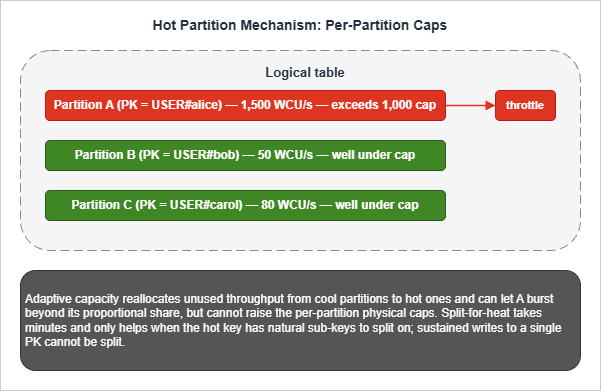

Hot Partition Mechanism: Per-Partition Caps

The first diagnostic: CloudWatch Contributor Insights for DynamoDB, an opt-in feature that lists the most-accessed PK and SK values per table. A single PK appearing as >50% of the traffic for sustained windows is a hot key. Throttling shows up in CloudWatch as ThrottledRequests, ReadThrottleEvents, and WriteThrottleEvents.

The AWS Database Blog series Scaling DynamoDB: How partitions, hot keys, and split for heat impact performance is the most thorough public explanation of the underlying mechanics, including the surprising result that LSIs prevent split-for-heat (because the partition cannot split without the LSI partition splitting in lockstep, and LSIs are pinned to the base partition).

5.2 Write Sharding — Random vs Calculated vs Calendar

The three write-sharding strategies are different trade-offs, not three forms of the same idea.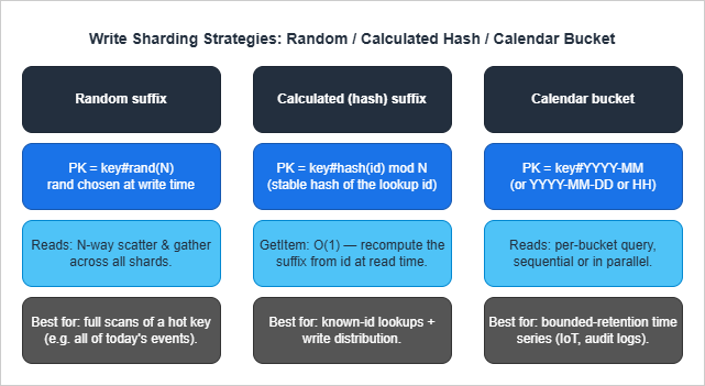

Write Sharding Strategies: Random / Calculated Hash / Calendar Bucket

Random suffix distributes writes uniformly but forces every read to fan out across all N shards. Use when reads are always full scans of the logical key (e.g., "all events for today").

Calculated (hash) suffix distributes writes uniformly and lets GetItem retrieve a known item in O(1) by recomputing the hash. Use when most reads target a known ID. The hash function must be stable (hash(orderId) % N works only if N never changes — see the AWS GSI Sharding for High-Cardinality Indexed Attributes for a worked example).

Calendar bucket (Pattern P10) bounds the per-PK item collection size by time and naturally distributes writes if the underlying entity is many devices each writing into their own bucket. Use for IoT and audit-log workloads.

The three are composable. A high-volume IoT pipeline might use PK = DEVICE#<id>#<YYYY-MM-DD>#<hash(eventId) % 4> — calendar bucket and per-device hash sharding within each bucket.

5.3 Read Sharding — Replicated Items and Scatter-Gather

Read sharding (Pattern P18) targets the 3,000 RCU/s read cap. The base item lives once in the table, but its position in a leaderboard or popularity ranking is replicated across N GSI partitions by setting a shard attribute. Reads scatter across shards, gather, merge.

The cost is double:

Storage: the GSI duplicates the projected attributes in every shard partition.
Per-read RCU: the read cost is proportional to N regardless of how many items are returned.

When read rate exceeds 3,000 RCU/s on a single PK and lower-latency caching (DAX, ElastiCache) is unavailable, read sharding is the only option. Otherwise, prefer DAX — it caches GetItem and Query results at microsecond latency without changing the schema.

5.4 Time Bucketing and Bounded Cardinality

Time bucketing (Pattern P10) is structurally a form of write sharding where the suffix is a time period. It additionally bounds item-collection growth, which matters when LSIs are present (10 GB ceiling) and when a Query(PK=...) would otherwise grow unboundedly.

A practical rule for picking bucket granularity:

Daily buckets when peak per-key writes are 100-1,000/s.
Hourly buckets when peak per-key writes are 1,000-10,000/s.
For sustained writes above 10,000/s on a single key, bucket and shard within bucket (PK = METRIC#<name>#<YYYY-MM-DD-HH>#<shard>).

For time series with bounded retention, also enable DynamoDB TTL to expire old buckets automatically. TTL deletes appear in DynamoDB Streams marked with userIdentity.principalId = "dynamodb.amazonaws.com", so archival Lambdas can distinguish retention deletes from user-initiated deletes.

5.5 Hot Partition Anti-Patterns

These designs create hot partitions and should never appear in production:

Monotonically increasing PK (PK = INVOICE#<auto_increment>) with high write rate — every write hits the most recent partition. Use ULID/KSUID instead.
Single global counter item without sharding (Pattern P20). The single item can only sustain ~1,000 WCU/s.
Single status value GSI partition (GSI1PK = "PENDING") when most items are pending. The constant key is a hot read partition.
Per-day PK (PK = "2026-05-06") with global write fan-in. Today's date is one partition. Either calendar-shard with a suffix or per-tenant calendar key.

6. Migration and Re-Keying Strategies

Re-keying — changing PK or SK schema — is the most operationally expensive change you can make to a live DynamoDB table. The reason is structural: DynamoDB has no ALTER TABLE for the primary key. A re-key requires a parallel-table migration with synchronization, validation, and a controlled cutover.

6.1 The Five-Step Online Re-Keying Procedure

This is the procedure that has worked across multiple production migrations, including the MuleSoft online migration on DynamoDB case study and AWS-recommended approaches.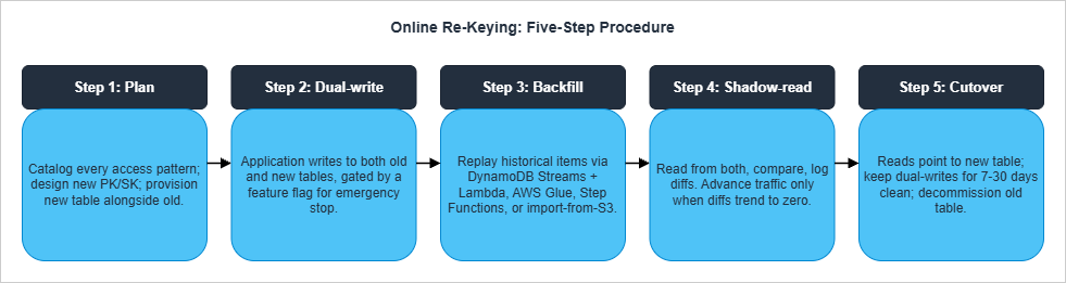

Step 1 — Plan. Catalog every existing query in the codebase (grep for query, get_item, scan). Group them by access pattern (not by table). Design the new key schema using the access-patterns worksheet from the Single Table Design guide. Provision the new table alongside the old.

Step 2 — Dual-write. Every mutation writes to both tables in the same Lambda or service. Wrap the dual-write behind a feature flag for emergency rollback. Fail closed: if either write fails, the request fails. Run for at least 24 hours to confirm no operational regressions.

Step 3 — Backfill historical data. Items that existed before dual-write turned on must be backfilled. Three options:

DynamoDB Streams + Lambda from the start (requires kicking off a Stream replay or ContinueProcessing for already-processed records — operationally tricky).
AWS Glue with the DynamoDB connector (best for tables under ~1 TB).
Step Functions distributed map over a parallel Scan (best for large tables, lets you tune parallelism).
DynamoDB import from S3 for an export-import path: export to S3 (point-in-time export), transform offline, import to a new table.

For very large migrations (multi-TB to PB scale) a common pattern is to track per-shard migration progress in a dedicated metadata table, fronted by an in-memory cache (DAX or ElastiCache) so the orchestration layer does not throttle the source or destination tables with status reads. Plan for at-least-once execution: every shard worker must be able to safely re-process records it has already migrated.

Step 4 — Shadow-read. In a controlled subset of traffic (1% → 10% → 50% → 100%), read from both tables and compare results. Log all diffs. Do not advance the percentage until diffs trend to zero. Common diff sources: timing (item updated between the two reads), missing backfilled items, type coercion bugs in transformation code.

Step 5 — Cutover. Switch reads to point only at the new table. Continue dual-writing for at least one full retention cycle (7-30 days depending on your audit requirements) so you can roll back if a regression is discovered. Stop dual-writes. Decommission the old table — but keep an export in S3 for at least one quarter.

6.2 Backfill Choice Matrix

* You can sort the table by clicking on the column name.

Backfill mechanism	Best for	Caveat
DynamoDB Streams + Lambda	Tables <100 GB; live at start of migration	Stream is 24 h retention only; not for re-runs
AWS Glue + DynamoDB connector	Tables <1 TB; one-time analytic-style transform	Provisioned capacity needs sizing; slow on huge tables
Step Functions distributed map + parallel Scan	Large tables; need fine-grained parallelism control	Scan cost is real; rate-limit to avoid base-table throttling
Export to S3 → transform → Import from S3	Tables >1 TB; offline transformation	No throughput consumed on the source table; new table is created from the import (cannot import into an existing table)

6.3 GSI Changes — Add and Remove

Unlike re-keying the primary key, GSI changes are online operations:

Add a GSI: backfill is automatic; the GSI becomes available when status reaches ACTIVE. Costs WCU on the GSI partition during backfill, so provision the new index generously (or use on-demand) to avoid extending the build time. Backfill duration scales with table size and is typically the dominant cost of the operation.
Delete a GSI: a metadata operation; immediate. The GSI's storage is reclaimed.
Change a GSI's projection: not directly supported. You must add a new GSI with the desired projection and then delete the old one. The transitional period costs double GSI storage.

When designing the table on day one, leave one or two "reserve" GSI slots (GSI1, GSI2, GSI3) free for future overload patterns. Adding a GSI later is cheap; designing the schema to not need one is cheaper still.

6.4 Common Re-Key Pitfalls

Forgetting reserved attributes. When the new schema introduces GSI1PK, GSI1SK, Type, items must have these attributes from the start of dual-write or the GSI will be sparse in unintended ways.
Type coercion in transforms. DynamoDB has typed attributes (S for string, N for number). Transforming userId = 123 (number) to PK = "USER#123" (string) is a type change that often breaks deserialization on the read side.
TTL changes mid-migration. Migrating items past their TTL during dual-write quietly drops them.
Stream backlog during cutover. Cutover under heavy stream load can leave the new table behind the old by minutes. Pause at low-traffic windows.

7. Anti-Patterns Catalog

A summary of the design choices that look reasonable and fail in production. Each has been covered in context above, gathered here for reference.
* You can sort the table by clicking on the column name.

#	Anti-Pattern	Why It Fails	Better Approach
A1	Sequential numeric PK from a centralized counter (`USER#0001`, `USER#0002` ...)	Requires a global counter as a single writer; IDs are predictable and trivially enumerable; PK carries no embedded metadata	ULID, KSUID, UUIDv7, or hashed natural key
A2	No type prefix (`PK = "u_001"`)	Cannot mix entity types in a single table; debug is painful	Always prefix (`USER#`, `ORDER#`)
A3	`PK = current_date`	Today's PK is hot for the whole day	Calendar shard with suffix (Pattern P17)
A4	`Scan` in production code paths	Every read is full-table; cost scales with size	`Query` against an index designed for the access pattern
A5	`FilterExpression` for >10% of items	Filter runs after RCU is consumed	Redesign keys so filter is unnecessary
A6	LSI to "improve query flexibility"	10 GB cap activates; cannot be removed; prevents split-for-heat	GSI
A7	One GSI per access pattern	20-GSI ceiling; storage cost grows linearly	Overload GSIs (Section 3.3)
A8	Single global counter item	1,000 WCU/s ceiling	Sharded counter (Pattern P20)
A9	Constant GSI PK on 80% of items	Hot read partition on the GSI	Time-bucket the GSI key
A10	Reading after write through a GSI	GSI is eventually consistent	Read base table with `ConsistentRead=True`
A11	No `ConditionExpression` on FSM transitions	Invalid state transitions silently succeed	Always condition on expected current state
A12	`TransactWriteItems` for all multi-item writes	2× WCU cost	Use only when invariants must hold across items
A13	Storing large blobs in DynamoDB	400 KB item ceiling; full item rewrite per update	Pointer to S3
A14	`BatchWriteItem` without retry on `UnprocessedItems`	Partial failures silently lost	Always retry with exponential backoff
A15	Unbounded item collection per PK	Performance degrades; LSI 10 GB ceiling	Time-bucket or split into child table
A16	TTL for correctness-critical deletion	Up to 48 h lag	Filter on status attribute and use TTL only for storage cleanup
A17	`ConsistentRead=True` everywhere	2× RCU; rejected on GSIs	Use only when the read-after-write boundary requires it
A18	Forgetting `Type` attribute on overloaded items	Stream consumers cannot route updates; debug pain	Set `Type` on every item

8. Summary — The Decision Order

When in doubt, follow this order — every step depends on the previous:

Access patterns. Enumerate every read and write in plain English before drawing any keys. If a pattern requires Scan or FilterExpression on a large fraction of items, redesign the access pattern before redesigning the keys.
PK schema. Choose a high-cardinality, evenly-distributed PK with a type prefix. If a single logical entity exceeds 1,000 WCU/s or 3,000 RCU/s, plan write-sharding or read-sharding into the design from day one.
SK schema. Decide hierarchical, composite, or sortable based on the dominant range query. Use type-prefixed SK segments (ORDER#, EVENT#, ADDR#).
GSIs. Design the minimum GSIs that serve the remaining access patterns, prefer overloading over per-pattern indexes, leave 2-3 reserve slots, and accept eventual consistency.
LSIs. Use only when strong consistency on an alternate sort is required and item collections are guaranteed under 10 GB forever.
Sharding. Pre-plan write/read sharding for any entity with hot-partition risk. Pick N = ceil(peak_load / per_partition_cap).
Code. Implement against the access-pattern catalog. Treat any design drift (Scan in prod, FilterExpression on majority, dynamic key construction in app code) as a code review failure.

The single most expensive change is changing PK/SK after launch (Section 6). Spend on the design pass; save on the migration. The patterns in Section 4 are the building blocks. Your real schema is a composition of three to seven of them.