Amazon DynamoDB Single Table Design Complete Guide - Access-Pattern-Driven Data Modeling Patterns
First Published:
Last Updated:
This article walks through how to redesign DynamoDB schemas around access patterns first using the Single Table Design approach. We will cover the core building blocks (Partition Key, Sort Key, Item Collection, and GSI sparse indexes), then walk through five concrete modeling patterns with PK/SK layouts and Python
boto3 code, and finish with a practical migration approach, common pitfalls, and tooling.This is a companion piece to the broader AWS database comparison in Summary of Differences and Commonalities in AWS Database Services using the Quorum Model, focused specifically on practical DynamoDB modeling.
1. Why Single Table Design — The Problem It Solves
In a multi-table design, fetching "a user with their last 10 orders, their default shipping address, and the items in those orders" typically requires 3–4 round-trips and application-side joins. In DynamoDB, each request has fixed per-call latency, fixed per-call cost (RCU/WCU), and a separate connection budget. Multi-table designs amplify all three.Single Table Design (STD) compresses related entities into one table by using overloaded keys so that a single
Query returns an entire item collection (a hierarchical slice of related items). Properly designed, the most common screens of an application can be served by one or two queries instead of four to ten.Three concrete benefits:
- Latency — one network round-trip for an entire screen's data.
- Cost — fewer RCUs because related items live on the same partition and arrive in a single read.
- Operations — one table's capacity, alarms, backups, and IAM policies to manage instead of N.
2. Core Concepts You Must Internalize
2.1 Partition Key, Sort Key, and Item Collection
A DynamoDB primary key is either a single Partition Key (PK) or a composite of PK + Sort Key (SK). All items sharing the same PK form an item collection, sorted by SK. AQuery operation reads one item collection at a time and supports range conditions on SK (=, begins_with, between, <, >, <=, >=).The whole point of STD is to put related entities into the same item collection and distinguish them with prefixed SK values like
PROFILE, ORDER#2026-04-26#abc, ADDR#home. The shape of an item collection is best understood visually: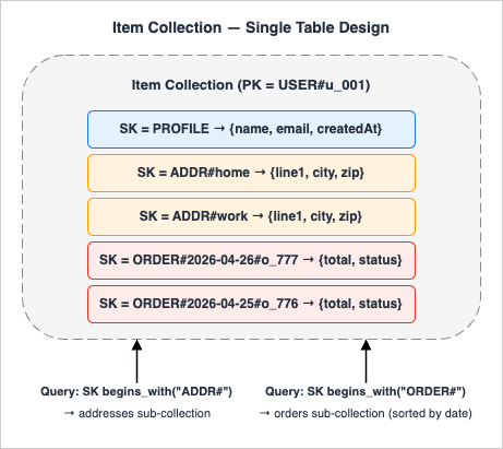
A single
Query can fetch any sub-collection (profile, addresses, or orders) in one round-trip without a join, and GetItem targets the specific (PK, SK) pair when only one item is needed.2.2 Global Secondary Index (GSI) and Sparse Index
A GSI is an alternative indexed view of the same table that DynamoDB maintains automatically. It can use a partition-key-only schema or a composite(PK, SK) schema, and may project a subset of attributes (see "GSI storage cost" in Section 10). Two important uses:- Inverse index — swap PK/SK to support the opposite query direction (e.g., "find all users in a group" when the base table answers "find all groups for a user").
- Sparse index — only items that contain the GSI's PK attribute are indexed. This makes a GSI act as a filtered view (e.g., only
STATUS=OPENorders).
GSI vs LSI: A Local Secondary Index (LSI) shares the base table's PK but allows a different SK, so it provides an alternative sort order within the same item collection. A Global Secondary Index (GSI) uses an entirely different
(PK, SK) pair, so it can repartition the data along an unrelated axis. LSIs must be defined at table creation and force the base table into a 10 GB-per-item-collection limit; GSIs can be added later, can be sparse, and have no item-collection size limit. Single Table Design typically uses GSIs because most cross-entity queries cut across partitions; LSIs are useful only when you need a second SK ordering (e.g. by updatedAt) without leaving the same partition.2.3 Generic Key Names and Type Attribute
To overload a single table, use generic attribute names (PK, SK, GSI1PK, GSI1SK) rather than entity-specific ones (UserId, OrderId). Add a Type attribute (USER, ORDER, ADDRESS) to make items self-describing for debugging and stream consumers.3. Pattern 1: One-to-Many with a Hierarchical Sort Key
Use case: A user has a profile, multiple addresses, and multiple orders. Access patterns:- P1: Get user profile by user ID via
GetItem— cheaper than scanning the item collection when only the profile is needed. - P2: Get all addresses for a user in a single
Query. - P3: Get the latest N orders for a user.
3.1 Key Design
| PK | SK | Type | Attributes |
|---|---|---|---|
USER#u_001 | PROFILE | USER | name, email, createdAt |
USER#u_001 | ADDR#home | ADDRESS | line1, city, zip |
USER#u_001 | ADDR#work | ADDRESS | line1, city, zip |
USER#u_001 | ORDER#2026-04-26#o_777 | ORDER | total, status |
USER#u_001 | ORDER#2026-04-25#o_776 | ORDER | total, status |
Because orders embed an ISO-8601 timestamp in the SK, they sort newest-last (or newest-first when
ScanIndexForward=False) without a separate index.3.2 Query Code
import boto3
from boto3.dynamodb.conditions import Key

ddb = boto3.resource("dynamodb")
table = ddb.Table("AppTable")

# P1: profile only
profile = table.get_item(
    Key={"PK": "USER#u_001", "SK": "PROFILE"}
).get("Item")

# P2: all addresses for the user (one Query, SK prefix)
resp = table.query(
    KeyConditionExpression=Key("PK").eq("USER#u_001")
        & Key("SK").begins_with("ADDR#"),
)
addresses = resp["Items"]

# P3: latest 10 orders
resp = table.query(
    KeyConditionExpression=Key("PK").eq("USER#u_001")
        & Key("SK").begins_with("ORDER#"),
    ScanIndexForward=False,
    Limit=10,
)
recent_orders = resp["Items"]
between("ADDR#", "ADDR$") trick: An alternative bounded form is between("ADDR#", "ADDR$"), which works because $ (0x24) is the next ASCII codepoint after # (0x23), keeping the query cleanly bounded to the address sub-collection. It is safe only when no SK in the table starts with ADDR$ (or any byte sequence whose first non-ADDR codepoint sits between 0x23 and 0x24 inclusive) — in practice that means ASCII-only suffixes with no shell metacharacters. For SKs that may include non-ASCII or arbitrary user input, stick with begins_with("ADDR#") as shown above.4. Pattern 2: Many-to-Many with the Adjacency List Pattern
Use case: Users belong to many groups; groups contain many users. Access patterns:- P4: List all groups a user belongs to.
- P5: List all users in a group.
4.1 Key Design
Store the relationship from both directions, plus a GSI for the inverse query.| PK | SK | GSI1PK | GSI1SK | Type |
|---|---|---|---|---|
USER#u_001 | GROUP#g_42 | GROUP#g_42 | USER#u_001 | MEMBERSHIP |
USER#u_001 | GROUP#g_99 | GROUP#g_99 | USER#u_001 | MEMBERSHIP |
USER#u_002 | GROUP#g_42 | GROUP#g_42 | USER#u_002 | MEMBERSHIP |
4.2 Query Code
# P4: groups for a user
resp = table.query(
    KeyConditionExpression=Key("PK").eq("USER#u_001")
        & Key("SK").begins_with("GROUP#"),
)

# P5: users in a group (via GSI1)
resp = table.query(
    IndexName="GSI1",
    KeyConditionExpression=Key("GSI1PK").eq("GROUP#g_42")
        & Key("GSI1SK").begins_with("USER#"),
)
(PK, SK) = (USER, GROUP) and GSI1 indexes (GSI1PK, GSI1SK) = (GROUP, USER). There is no duplication of the relationship — only an index of it.5. Pattern 3: Time-Series with GSI Inverse and Composite Sort Key
Use case: IoT devices emit events. Access patterns:- P6: Latest events for a given device.
- P7: All events of a given event type within a time range, across devices.
5.1 Key Design
| PK | SK | GSI1PK | GSI1SK |
|---|---|---|---|
DEVICE#d_001 | EVT#2026-04-26T10:15:00Z#e_abc | EVTTYPE#TEMP_HIGH | 2026-04-26T10:15:00Z#d_001 |
DEVICE#d_001 | EVT#2026-04-26T10:14:55Z#e_abd | EVTTYPE#HEARTBEAT | 2026-04-26T10:14:55Z#d_001 |
Embedding the ISO-8601 timestamp in the SK makes time-range queries trivial. The GSI flips the perspective: by event type, sorted by timestamp.
5.2 Query Code
# P6: device events in the last hour
from datetime import datetime, timedelta, timezone
now = datetime.now(timezone.utc)
end = now.strftime("%Y-%m-%dT%H:%M:%SZ")
start = (now - timedelta(hours=1)).strftime("%Y-%m-%dT%H:%M:%SZ")

resp = table.query(
    KeyConditionExpression=Key("PK").eq("DEVICE#d_001")
        & Key("SK").between(f"EVT#{start}", f"EVT#{end}~"),
)

# P7: all TEMP_HIGH events today (across devices)
resp = table.query(
    IndexName="GSI1",
    KeyConditionExpression=Key("GSI1PK").eq("EVTTYPE#TEMP_HIGH")
        & Key("GSI1SK").begins_with("2026-04-26"),
)
GSI1PK with a write-shard suffix (EVTTYPE#TEMP_HIGH#0..#9) and fan out reads across shards to avoid hot partitions on a single event type.Note: Fan-out reads require N parallel
Query operations (one per shard suffix #0..#9), then application-side merge — read RCU consumption multiplies by the shard count and merging adds latency. Adaptive Capacity automatically absorbs short-term partition bursts but does not eliminate the need for sharding for sustained hot workloads.TTL for time-series retention: For event streams with bounded retention (e.g. 90 days), enable DynamoDB TTL on a numeric epoch attribute (
expiresAt). DynamoDB deletes expired items asynchronously at no extra cost, and the deletes appear in DynamoDB Streams so downstream consumers can react. TTL-driven deletes are distinguishable from user-initiated DeleteItem calls in the stream record by inspecting userIdentity: a TTL delete carries userIdentity = { "type": "Service", "principalId": "dynamodb.amazonaws.com" }, which lets archival Lambdas filter precisely on retention deletes. Note TTL deletes are best-effort within 48 hours; design queries to filter on expiresAt if a strict cutoff is required.6. Pattern 4: Hierarchical Data (Tree / Materialized Path)
Use case: An organizational tree, a category taxonomy, or a tag hierarchy. Access patterns:- P8: Get a node and its direct children.
- P9: Get an entire subtree (all descendants).
6.1 Key Design — Materialized Path
Store each node's full path from the root in the SK so prefix queries return entire subtrees.| PK | SK | Type | Name |
|---|---|---|---|
ORG#root | PATH#root | NODE | Acme Inc. |
ORG#root | PATH#root#eng | NODE | Engineering |
ORG#root | PATH#root#eng#cloud | NODE | Cloud Team |
ORG#root | PATH#root#eng#cloud#aws | NODE | AWS Squad |
ORG#root | PATH#root#sales | NODE | Sales |
6.2 Query Code
# P9: entire subtree under Engineering
resp = table.query(
    KeyConditionExpression=Key("PK").eq("ORG#root")
        & Key("SK").begins_with("PATH#root#eng"),
)

# P8: direct children of Engineering only
# (post-filter by depth = 3 segments)
children = [
    item for item in resp["Items"]
    if item["SK"].count("#") == 3
]
Depth attribute and index it as GSI1PK = ORG#root#depth=3 for an O(1) child listing.Hot partition warning: Because every node shares
PK = ORG#root, the entire tree lives in a single item collection. This is fine for tens of thousands of nodes but breaks down for very large trees: writes concentrate on one partition, and any LSI defined at table-creation time imposes the 10 GB-per-item-collection limit on the entire tree (LSIs cannot be added after the table is created). For multi-tenant or large taxonomies, partition by tenant or top-level subtree (PK = ORG#<tenant_id> or PK = ORG#<top_level_dept>) so each tree gets its own partition.7. Pattern 5: Geospatial with Geohash + GSI
Use case: "Find shops within ~1 km of a user's current location." Access patterns:- P10: Find points of interest near a (lat, lng) pair.
7.1 Key Design — Geohash Bucketing
Compute a geohash (e.g., precision 6 ≈ 1.2 km × 0.6 km cell) for each point and use it as the GSI partition key. The GSI sort key carries the precise coordinates and the entity ID for tie-breaking.| PK | SK | GSI1PK | GSI1SK |
|---|---|---|---|
SHOP#s_001 | META | GEO#xn774c | 35.6586#139.7454#s_001 |
SHOP#s_002 | META | GEO#xn774c | 35.6595#139.7460#s_002 |
SHOP#s_003 | META | GEO#xn774b | 35.6500#139.7400#s_003 |
7.2 Query Code
# P10: shops in geohash cell xn774c
resp = table.query(
    IndexName="GSI1",
    KeyConditionExpression=Key("GSI1PK").eq("GEO#xn774c"),
)
# Then post-filter by precise haversine distance.
dynamodb-geo (Java, Node; an AWS Labs project with sporadic maintenance) and python-geohash (a general-purpose geohash encoder, not DynamoDB-specific) cover the boilerplate. For variable radius, query at multiple geohash precisions and dedupe.7.3 Fan-out Reads with asyncio
Both the geohash neighbor query and the write-shard pattern from Section 5 require N parallel Query calls followed by an application-side merge. The cleanest implementation uses asyncio with aioboto3 (or concurrent.futures.ThreadPoolExecutor for synchronous code):import asyncio
import aioboto3
from boto3.dynamodb.conditions import Key
async def query_one(table, gsi1pk):
resp = await table.query(
IndexName="GSI1",
KeyConditionExpression=Key("GSI1PK").eq(gsi1pk),
)
return resp["Items"]
async def fan_out_geohash(center_cell, neighbor_cells):
session = aioboto3.Session()
async with session.resource("dynamodb") as ddb:
table = await ddb.Table("AppTable")
cells = [center_cell, *neighbor_cells]
results = await asyncio.gather(
*(query_one(table, f"GEO#{c}") for c in cells)
)
# Flatten, then haversine-filter in application code
return [item for sublist in results for item in sublist]
8. Production Essentials: Pagination, Conditional Writes, and Consistency
The five patterns above cover the read shape, but every production codebase also needs to handle pagination, concurrent updates, and consistency carefully. These three concerns trip up otherwise solid designs.8.1 Pagination with LastEvaluatedKey
DynamoDB caps a single Query or Scan response at 1 MB. Beyond that, the response includes a LastEvaluatedKey that you pass back as ExclusiveStartKey on the next call. The Limit parameter caps the number of items examined (not returned after filter), so a query with a FilterExpression may return fewer items than Limit while still being paginated.def query_all(table, pk_value, sk_prefix):
items = []
last_key = None
while True:
kwargs = {
"KeyConditionExpression": Key("PK").eq(pk_value)
& Key("SK").begins_with(sk_prefix),
}
if last_key:
kwargs["ExclusiveStartKey"] = last_key
resp = table.query(**kwargs)
items.extend(resp["Items"])
last_key = resp.get("LastEvaluatedKey")
if not last_key:
break
return items
LastEvaluatedKey dictionary — serialize it (base64 of JSON, or a signed JWT) so the cursor remains opaque and tamper-resistant. Two pitfalls:- An empty result page with a non-null
LastEvaluatedKeyis normal — do not treat it as "end of data." - For UI "jump to page 50" patterns, DynamoDB does not support offset-based paging. Either restrict UX to next/prev cursors, or maintain a separate counter table.
8.2 Conditional Writes and Optimistic Locking
ConditionExpression on PutItem, UpdateItem, DeleteItem, and TransactWriteItems evaluates server-side at no extra RCU cost (a failed condition still consumes 1 WCU). Two common uses:(a) Idempotent insert — refuse to overwrite an existing item:
from botocore.exceptions import ClientError

try:
    table.put_item(
        Item={"PK": "USER#u_001", "SK": "PROFILE", "name": "Alice"},
        ConditionExpression="attribute_not_exists(PK)",
    )
except ClientError as e:
    if e.response["Error"]["Code"] == "ConditionalCheckFailedException":
        # Item already exists — idempotent no-op
        pass
    else:
        raise
version attribute and increment it only if the read-time version still matches:def update_with_version(table, pk, sk, expected_version, new_total):
table.update_item(
Key={"PK": pk, "SK": sk},
UpdateExpression="SET #t = :total, version = version + :one",
ConditionExpression="version = :expected",
ExpressionAttributeNames={"#t": "total"},
ExpressionAttributeValues={
":total": new_total,
":expected": expected_version,
":one": 1,
},
)
ConditionalCheckFailedException and must re-read, recompute, and retry. This avoids the lost-update problem without a distributed lock.(c) When to step up to
TransactWriteItems — conditional UpdateItem handles the single-item case, but ACID guarantees across multiple items (e.g. debit account A and credit account B atomically, or insert an order while decrementing inventory) require TransactWriteItems. It supports up to 100 actions and a 4 MB total payload per transaction, accepts a per-action ConditionExpression, and consumes 2× the WCU of an equivalent batched non-transactional write — reserve it for cases where partial failure would corrupt invariants, not as a default for multi-item writes.8.3 Strong vs Eventually Consistent Reads
By default,GetItem, Query, and Scan on the base table are eventually consistent — cheaper (0.5 RCU per 4 KB) and lower latency. Pass ConsistentRead=True for strongly consistent reads (1 RCU per 4 KB, slightly higher latency, served only from the leader replica).- GSI reads are always eventually consistent;
ConsistentRead=Trueis rejected on a GSI. - Use strong consistency for read-after-write workflows on the same item (e.g., re-read after a transactional update). For most read paths, eventual consistency is the right default.
- LSIs do support
ConsistentRead=Truebecause they share the base table's partition. - Transactional reads (
TransactGetItems) provide a serializable snapshot across up to 100 items at a cost of 2 RCU per 4 KB per item (double a strongly-consistent read). Reach for them only when you genuinely need a consistent multi-item view (e.g. account balance + open holds) — for most screens, parallelBatchGetItemwith eventual consistency is dramatically cheaper.
# Strongly consistent read (re-read after a write to the same item)
profile = table.get_item(
    Key={"PK": "USER#u_001", "SK": "PROFILE"},
    ConsistentRead=True,
).get("Item")
9. The Access Patterns Worksheet
Before writing any keys, fill in this worksheet. The goal is to lock the read shape before the schema, because schema changes after launch are expensive in DynamoDB.| # | Access Pattern | Entry Entity | Filters / Range | Sort Direction | Frequency | Latency Budget |
|---|---|---|---|---|---|---|
| 1 | Get user profile by ID | User | – | – | very high | < 10 ms |
| 2 | List user's last 10 orders | User | last 30 days | newest first | high | < 30 ms |
| 3 | List shops near (lat, lng) | Geo | radius 1 km | – | medium | < 50 ms |
| 4 | Get all members of a group | Group | – | by join date | medium | < 30 ms |
Then for every row, write down the table or GSI that will serve it and the resulting
Query/GetItem call. If a row needs a Scan, that is a red flag — re-design.A practical rule from production: any pattern that requires
FilterExpression on more than 10% of items is a design smell. Filter expressions run after the read consumes RCU; they save bandwidth but not capacity.10. Migrating from Multi-Table to Single Table
You rarely get to start fresh. The migration path that has worked well in practice is incremental and read-first:- Catalogue every existing query in the codebase. Group them by access pattern, not by table.
- Design the new key schema (PK/SK/GSIs) on paper using the worksheet from Section 9.
- Provision the new table alongside the old ones.
- Dual-write on every mutation: write to both old and new tables in the same Lambda/service, fail closed if either write fails.
- Backfill historical items via a one-off job (Step Functions + parallel Scan, or AWS Glue).
- Shadow-read in production: read from both tables and compare. Log diffs.
- Cut over reads one pattern at a time, monitoring p99 latency and error rate.
- Stop dual writes and decommission the old tables.
11. Common Pitfalls
- Hot partitions. Sequential keys (
USER#0001,USER#0002...) all land on the same partition under heavy write load. Use high-cardinality identifiers (UUID, ULID) or write-sharding (USER#u_001#0..USER#u_001#9). - 400 KB item-size ceiling. Large blobs (full HTML, images, large JSON) belong in S3, with a pointer in DynamoDB. The 400 KB limit is hard.
- GSI storage cost. Every GSI duplicates indexed attributes. Choose the projection type deliberately:
ALL(full attribute set, highest cost),KEYS_ONLY(PK + SK only), orINCLUDE(selected attributes). UseKEYS_ONLYorINCLUDEwhenever the query does not need all attributes. - GSI / LSI quota ceilings. A single table can hold up to 20 GSIs and 5 LSIs by default. The GSI quota is adjustable via Service Quotas; the LSI quota is fixed because LSIs can only be created at table-creation time and cannot be added later. Plan the "reserve" GSIs (e.g.
GSI1–GSI3as generic overload indexes) explicitly. - Cross-partition transactions.
TransactWriteItemssupports up to 100 actions and a 4 MB total payload per transaction; its idempotency token (ClientRequestToken) is only honored for 10 minutes — design retries accordingly. On retry with the same token, DynamoDB returns the cached result of the prior transaction (success orIdempotentParameterMismatchException). If the prior call is still in flight, you may receiveTransactionInProgressException. - Batch API partial failures.
BatchWriteItemaccepts up to 25 items (16 MB max payload) and supports only Put and Delete — not Update.BatchGetItemaccepts up to 100 keys (16 MB max response). Both APIs return unprocessed items inUnprocessedItems/UnprocessedKeysrather than raising an exception; always check those fields and retry with exponential backoff:import time def batch_write_with_retry(table, requests, max_retries=5): remaining = requests for attempt in range(max_retries): resp = table.meta.client.batch_write_item( RequestItems={table.name: remaining} ) remaining = resp.get("UnprocessedItems", {}).get(table.name, []) if not remaining: break time.sleep(2 ** attempt * 0.1) # exponential backoff Scanin production code. AnyScanthat is not part of a one-off admin job is a bug.- GSI eventual consistency. GSIs are always eventually consistent; do not read-after-write through a GSI in the same logical operation.
- Forgotten
Typeattribute. Without it, stream consumers (DynamoDB Streams → Lambda) cannot route items, and on-call debugging at 3 AM becomes painful.
12. Tooling
- NoSQL Workbench for DynamoDB — a free desktop app from AWS for visualizing item collections, designing keys, and exporting CloudFormation/CDK definitions. Indispensable when communicating designs to teammates.
- DynamoDB Local — a self-contained JAR (or Docker image) for offline development and CI tests. Pair with
pytestandmotofor unit tests. - AWS CDK / Terraform — define the table, all GSIs, TTL attribute, point-in-time recovery, and contributor insights as code. Drift between environments is a frequent source of incident.
- Contributor Insights — an opt-in feature that surfaces the most-accessed partition keys; the fastest way to spot a hot partition.
- CloudWatch alarms — at minimum, alarms on
ThrottledRequests,SystemErrors, andUserErrorsper table and per GSI. - DynamoDB Accelerator (DAX) — an in-memory write-through cache that drops single-digit-millisecond reads to microseconds for read-heavy workloads. DAX maintains two distinct caches: an item cache for
GetItem/BatchGetItem(which target the base table by definition) and a query cache forQuery/Scanresults (against either the base table or a GSI). The cluster sits inside a VPC and writes are passed through synchronously, so DAX is most useful for repeatable hot read patterns rather than mutation-heavy or strongly-consistent workloads (DAX always returns eventually-consistent data even whenConsistentRead=Trueis requested — that flag transparently bypasses DAX). - PartiQL — a SQL-compatible query language supported by DynamoDB for
SELECT/INSERT/UPDATE/DELETE. Useful for ad-hoc console queries and onboarding RDBMS-fluent engineers, but it does not bypass the access-pattern-first discipline: aSELECTwithout a key condition still becomes a fullScanunder the hood. Treat it as syntactic sugar over the same primitives, not as a replacement for key design.
13. When NOT to Use Single Table Design
STD is not universally optimal. The trade-off is real: you exchange schema flexibility and team onboarding speed for runtime efficiency. Skip STD — or use a hybrid (a few logical tables, each internally overloaded) — when any of the following apply:- Analytics / OLAP workloads. Ad-hoc aggregations, group-by, and full-table scans are not what DynamoDB is for. Export to S3 via Point-in-Time Export and query with Athena or Redshift Spectrum.
- Rapidly evolving schema. If new entity types appear weekly and access patterns are still in flux, the up-front design cost of STD will be paid repeatedly. A multi-table design is more forgiving while the domain stabilizes; migrating to STD later is feasible (Section 10).
- Per-entity IAM scoping. When fine-grained IAM policies must restrict access at the entity level, separate tables give you separate ARNs to scope. STD requires
dynamodb:LeadingKeysconditions and is harder to audit. - Joins or cross-entity transactions across many entities. If business logic needs "join customer + invoice + line items + payments" with ad-hoc filters, an OLTP relational store (Aurora, RDS) is a better fit.
TransactWriteItemscaps at 100 actions per call. - Inexperienced team. STD requires fluency in access-pattern-first thinking. A team new to DynamoDB will ship faster with multi-table; the operational story is easier to debug.
- Heavy use of full-text search or geographic radius queries. Geohash gets you 80% of the way (Section 7) but is no substitute for OpenSearch, Aurora PostGIS, or Amazon Location Service when the search semantics are rich.
14. Summary
Single Table Design is not "the right way to use DynamoDB" in the abstract — it is the right way to use DynamoDB when latency, cost, and a finite query budget matter. The five patterns above (one-to-many with hierarchical SK, many-to-many adjacency list, time-series with GSI inverse, hierarchical materialized path, and geospatial geohash) cover the overwhelming majority of real workloads. Start from the access patterns, write the worksheet, then design the keys.When in doubt, the order of operations is: access patterns → key schema → GSIs → code. Never the other way around.
15. References
- Best Practices for Designing and Architecting with DynamoDB - AWS Documentation
- Best Practices for Modeling Relational Data in DynamoDB
- Best Practices for Managing Many-to-Many Relationships (Adjacency List)
- Using Global Secondary Index Overloading
- Best Practices for Handling Time Series Data in DynamoDB
- Choosing the Right DynamoDB Partition Key - AWS Database Blog
- Summary of Differences and Commonalities in AWS Database Services using the Quorum Model
- DynamoDB Capacity Calculator Tool
References:
Tech Blog with curated related content
Written by Hidekazu Konishi