hidekazu-konishi.com

Amazon DynamoDB Master Index - A Hub for DynamoDB Design, Key Modeling, and Capacity Planning Articles

First Published: 2026-05-16
Last Updated: 2026-05-16

This page is the master index for every Amazon DynamoDB article and tool on hidekazu-konishi.com. If you are exploring DynamoDB for the first time, deciding between Single Table Design and Multi Table Design, choosing between a Global Secondary Index (GSI) and a Local Secondary Index (LSI), or estimating Read Capacity Units (RCU) and Write Capacity Units (WCU) before launch, start here. Each section gives you a one-screen overview, a self-named decision framework called The DynamoDB Access Pattern Map, and direct links to the deep-dive articles and the interactive DynamoDB Capacity Calculator tool.

DynamoDB content on this site is organized into three complementary deep-dive articles plus one client-side capacity calculator. This master index ties them together with a shared vocabulary, a decision tree for single vs multi table, and a 5-quadrant access pattern map so you can locate the right reference quickly.

What is Amazon DynamoDB?

Amazon DynamoDB is a fully managed, serverless, key-value and document NoSQL database service from AWS, designed for single-digit millisecond latency at any scale. It removes operational overhead around provisioning, patching, replication, and backup, so application teams can model access patterns directly against a managed primitive instead of running database servers.

Unlike relational databases, DynamoDB is built around an access-pattern-first modeling discipline. You do not normalize data and then write queries on top of it; you enumerate every read and write your application performs, then design a Partition Key (PK) and Sort Key (SK) layout that satisfies all of them with constant-time lookups. Schema flexibility, automatic horizontal partitioning, and built-in multi-AZ replication are the foundation; the design challenge sits in keys, indexes, and capacity.

Key Attributes at a Glance

Attribute	Value
Service type	Key-value and document NoSQL
Consistency model	Eventually consistent (default) / Strongly consistent (per-request opt-in) / Transactional
Capacity modes	On-Demand / Provisioned (with optional auto-scaling)
Maximum item size	400 KB (per item, including all attribute names and values)
Global distribution	Global Tables (multi-Region active-active replication)
Backup	Point-in-Time Recovery (PITR, continuous up to 35 days) / On-demand backup
Time-to-Live	TTL on a designated numeric attribute (item-level expiration)
Streams	DynamoDB Streams (change data capture, 24-hour retention)
Secondary indexes	Global Secondary Index (GSI) / Local Secondary Index (LSI)
API surface	Query, Scan, GetItem, BatchGetItem, PutItem, UpdateItem, DeleteItem, TransactWriteItems, TransactGetItems, PartiQL
Caching layer	Amazon DynamoDB Accelerator (DAX) — in-VPC write-through cache with microsecond reads for read-heavy workloads

DynamoDB Architecture Overview

This section gives a one-screen mental model of how DynamoDB physically stores and retrieves items. If you only remember three things, remember: (1) every item lives on a partition chosen by a hash of the Partition Key, (2) items that share a Partition Key are stored together and ordered by Sort Key, and (3) capacity is allocated per partition, so hot keys cause throttling even when the table average looks healthy.

Partition Key, Sort Key, and Item Identity

Every DynamoDB item is identified by a primary key that is either a single Partition Key (PK) or a composite of a Partition Key and a Sort Key (PK+SK). The Partition Key is hashed to select which physical partition stores the item. Two items with the same Partition Key always land on the same partition, so a Query on PK = "user#123" returns all matching items with a single internal partition lookup and an in-order range scan of the Sort Key. This is the entire reason DynamoDB can serve point reads and small range queries in single-digit milliseconds — the work is bounded by partition-local I/O, not by table-wide scanning.

Hash Distribution and Adaptive Capacity

DynamoDB hashes Partition Keys to spread items uniformly across partitions. Each partition has a soft ceiling of 3,000 RCU and 1,000 WCU per second. If your traffic concentrates on a small number of Partition Key values — for example, a "global counter" item, a single "today's-date" key in a time-series table, or a celebrity user ID — the partition holding those values will throttle while the rest of the table sits idle. This is the hot partition problem. Adaptive Capacity automatically rebalances unused throughput to busy partitions and isolates hot partition keys, which mitigates but does not eliminate the issue. Designing keys so traffic spreads naturally is still the correct fix, and it is the central subject of the DynamoDB Key Design Dictionary article linked below.

Storage Model — Items, Attributes, and the 400 KB Limit

A DynamoDB table is a collection of items. An item is a collection of attributes. An attribute is a name-value pair where the value can be scalar (String, Number, Binary, Boolean, Null), document (List, Map), or set (StringSet, NumberSet, BinarySet). Items in the same table are not required to share the same attributes — this schemaless property is what makes Single Table Design feasible (you can store users, orders, and order lines as differently-shaped items in one table). The 400 KB limit applies per item, including attribute names, so you should not store large blobs inline. Use Amazon S3 for the blob and store the S3 key as a DynamoDB attribute when an attribute would otherwise exceed the limit.

Read/Write Capacity Modes — Provisioned vs On-Demand

DynamoDB bills throughput in two modes. Provisioned mode requires you to declare RCU and WCU per table (or per GSI) up-front and supports auto-scaling between configured min/max bounds. It is cheaper per request at steady, predictable traffic. On-Demand mode bills per request with no capacity declaration, ideal for unpredictable spikes and new applications without a traffic baseline. The break-even point depends on utilization, and choosing the wrong mode for your workload can substantially change your DynamoDB bill. Use the DynamoDB Capacity Calculator tool linked below to estimate both modes side-by-side before committing.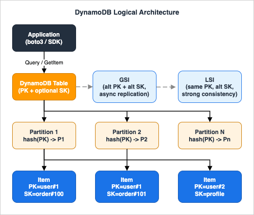

The DynamoDB Access Pattern Map (Self-Named Framework)

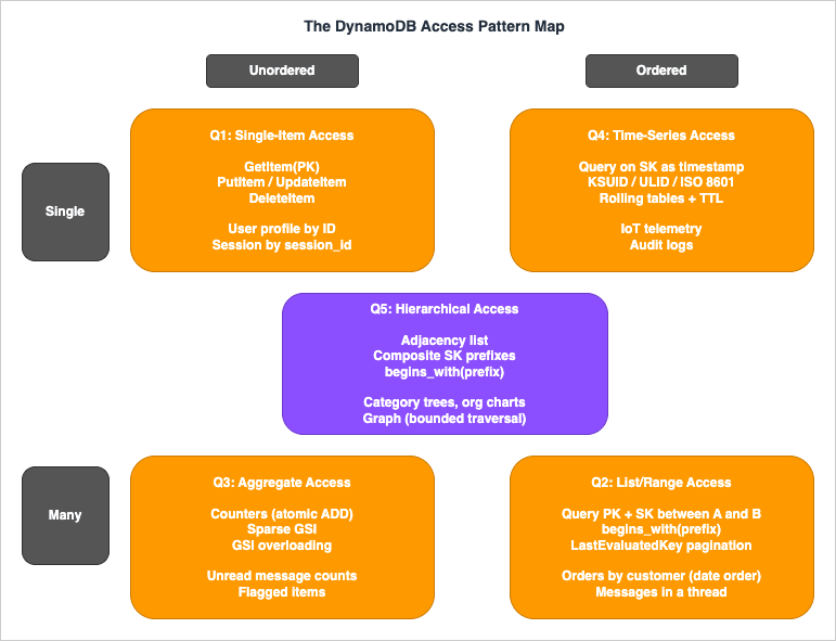
When teams stall on DynamoDB modeling, the symptom is almost always the same: they jump to "should this be one table or many?" before they have written down the actual access patterns. This master index introduces a framework — The DynamoDB Access Pattern Map — for classifying every read and write your application performs into one of five quadrants. Once each access pattern is placed on the map, key design and table strategy follow mechanically.

The map has two axes:

• Ordering axis (horizontal): is the result an unordered point/set or an ordered range?
• Cardinality axis (vertical): does the dominant operation touch a single item (point read/write or single append) or many items (range scan, batch, or aggregate) per call?

The five quadrants cover every meaningful DynamoDB access pattern.

Q1: Single-Item Access (Unordered, Single)

Point reads and point writes by primary key. GetItem(PK), PutItem, UpdateItem, DeleteItem. Examples: load a user profile by user ID, update a session record by session ID, fetch a feature flag by flag name. Key design: choose a Partition Key with high cardinality and even traffic distribution. No Sort Key required unless the entity has variants. This is the cheapest and fastest DynamoDB pattern and should be the first thing you map.

Q2: List/Range Access (Ordered, Many)

Query on PK = X AND SK BETWEEN A AND B or SK begins_with(prefix). Examples: list all orders for a customer in date order, fetch all messages in a chat thread after a given timestamp, list all line items belonging to a single order. Key design: use a composite Partition Key + Sort Key where the Partition Key isolates the entity and the Sort Key encodes the ordering dimension (timestamp, version, sequence). Pagination is handled by LastEvaluatedKey. This quadrant is where DynamoDB feels most relational-like.

Q3: Aggregate Access (Unordered, Many)

Counters, sparse indexes, and "find me everything that matches a flag" queries. Examples: count unread messages per user, fetch all orders currently in "pending" status, find every item with a non-null archived_at attribute. Key design: store a counter as a separate item updated with ADD on a numeric attribute (use atomic counters with care under high concurrency — multiple sub-counters with periodic aggregation avoid the hot-partition trap). For "find by flag" use a sparse GSI where the GSI Partition Key attribute is only set on items that match — non-matching items are not projected into the index at all.

Q4: Time-Series Access (Ordered by time, often append-heavy)

Sensor data, audit logs, event streams, append-only history. Examples: IoT telemetry, application logs, e-commerce clickstream. Q4 is positioned at Single + Ordered because the defining workload is single-item appends written in time-sorted order; range reads over the same time series belong to Q2. Key design: encode the time dimension into the Sort Key with lexicographically sortable timestamps (ISO 8601, KSUID, or ULID — never raw UNIX seconds, which can collide within the same second under burst traffic). For append-heavy workloads, consider rolling tables (one table per day or per month) so old data can be dropped by deleting an entire table — orders of magnitude cheaper than per-item deletes. Combine with TTL to expire individual items if rolling tables are too coarse-grained.

Q5: Hierarchical Access (Tree or graph structure)

Parent-child relationships, organizational charts, comment threads, category trees, adjacency lists, graph traversal. Examples: nested categories, file system directories, friend-of-friend lookups, multi-tenant resource hierarchies. Key design: use the adjacency list pattern where each edge is stored as an item with PK = node_id and SK = related_node_id, optionally with a type attribute distinguishing parent-of vs child-of vs sibling-of edges. Composite Sort Keys with delimiter-separated prefixes (org#region#site#asset) enable hierarchical queries via begins_with. Most graph-like patterns can be served by DynamoDB without moving to Amazon Neptune as long as traversal depth is bounded.

Quadrant-to-Article Mapping

Each quadrant maps to a deep-dive article on this site.

Quadrant	Primary deep-dive
Q1: Single-Item Access	DynamoDB Key Design Dictionary (PK selection, hot partition avoidance)
Q2: List/Range Access	Single Table Design Complete Guide (Sort Key patterns)
Q3: Aggregate Access	DynamoDB Key Design Dictionary (sparse GSI, counter sharding)
Q4: Time-Series Access	Single Table Design Complete Guide (time-series section)
Q5: Hierarchical Access	Single Table Design Complete Guide (adjacency list section)

Decision Tree — Single Table vs Multi Table

Once you have placed each access pattern on the map, the Single Table vs Multi Table question collapses to a small decision tree. The tree below walks through the yes/no checks that matter in practice. If you answer "yes" to the first two checks and either branch below them resolves to Single Table, Single Table Design is correct. If the first check answers "no", Multi Table Design (one entity per table) is correct. Mixed answers point to a hybrid where related entities share a table and unrelated ones do not.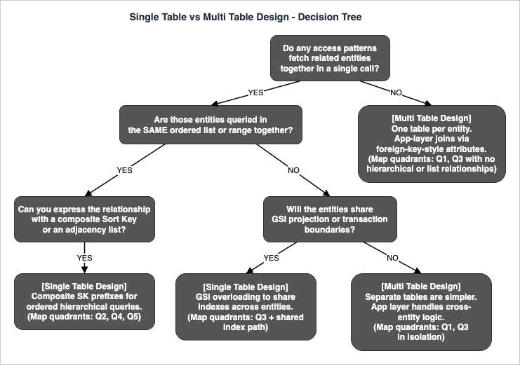

The takeaway: Single Table Design is correct when access patterns either bundle related entities into the same query or share the same GSI projections. Multi Table Design is correct when entities are independent — when there is no query that fetches them together and no transaction that updates them atomically. Most real applications end up with a small number of single tables (one per bounded context in DDD terms) rather than either extreme.

For the full decision matrix including conditional writes, transactions, and migration costs, see the Single Table Design Complete Guide linked below.

Deep Dive Articles

The four articles below are the substance of the DynamoDB content on this site. Read them in order if you are new to DynamoDB; jump directly if you have a specific question.

History and Timeline of Amazon DynamoDB

→ AWS History and Timeline regarding Amazon DynamoDB - Overview, Functions, Features, Summary of Updates, and Introduction

The DynamoDB timeline article traces the service from its 2012 launch through Global Tables, On-Demand mode, PITR, transactions, PartiQL support, and standard infrequent-access table class. If you need to know when a specific capability shipped — for example, "when did Global Tables go GA in their current form?" — that article is the reference. For the latest announcements that may post-date this index, the AWS What's New (Database) feed is the authoritative source.

Single Table Design Complete Guide

→ Amazon DynamoDB Single Table Design Complete Guide - Access-Pattern-Driven Data Modeling Patterns

The Single Table Design guide is the longest and most practice-oriented article in this series. It walks through the access-pattern-first methodology end-to-end: how to enumerate every read and write the application performs, translate them into key design, and represent multiple entity types in one table without normalization. It covers all five common patterns — one-to-many, many-to-many, time-series, hierarchical, and geospatial — with concrete Partition Key + Sort Key schemas and Python boto3 code.

The article also addresses the harder parts that most introductions skip: pagination with LastEvaluatedKey across composite keys, conditional writes to enforce uniqueness constraints, GSI projection strategies (KEYS_ONLY vs INCLUDE vs ALL) and their cost implications, and online migration procedures when an existing application needs to move from multi table to single table without downtime.

Read this article when you are designing a new DynamoDB table and need a step-by-step methodology. Quadrants Q2, Q4, and Q5 of the Access Pattern Map are covered in detail here.

DynamoDB Key Design Dictionary (PK/SK/GSI/LSI)

→ DynamoDB Key Design Dictionary: PK/SK, GSI/LSI Selection, Hot Partition Avoidance, and Re-Keying Patterns

The Key Design Dictionary is a reference-style article organized as a dictionary of named patterns. It covers the GSI vs LSI decision matrix (when to use which, and the irreversibility trap of LSI selection at table creation time), hot partition avoidance via write sharding (suffixing the Partition Key with a random shard ID) and read sharding (fan-out reads across the shards), and online re-keying procedures for when your Partition Key choice turns out to be wrong in production.

A few of the patterns documented: the sparse GSI pattern for "find all items with a flag set", the GSI overloading pattern where one GSI serves multiple unrelated query types by reusing the same attribute names with different semantics per item type, and the inverted index pattern where you swap PK and SK in a GSI to query the relationship from the opposite direction.

Read this article when you have a Single Table layout in mind but are choosing between GSI and LSI, or when you are debugging a hot-partition incident. Quadrants Q1 and Q3 of the Access Pattern Map are covered in detail here.

AWS Database Quorum Model Comparison

→ Summary of Differences and Commonalities in AWS Database Services using the Quorum Model - Comparison Charts of Amazon Aurora, Amazon DocumentDB, and Amazon Neptune

This article steps back from DynamoDB specifically and compares how AWS database services achieve durability and consistency. DynamoDB itself does not use the same quorum model as Aurora, DocumentDB, and Neptune — DynamoDB uses a Paxos-based three-AZ replication scheme for its underlying storage, with consistency exposed to the application as eventually consistent (default), strongly consistent (one extra round trip), or transactional (two-phase commit).

The comparison article details how Aurora, DocumentDB, and Neptune share a 6-copy / 4-of-6 write quorum / 3-of-6 read quorum design layered over a shared-storage architecture, and how that differs from DynamoDB's per-partition replication. If you are choosing between DynamoDB and one of the quorum-based AWS databases, this article gives you the conceptual scaffolding for the consistency and durability comparison.

Read this article when you are deciding whether DynamoDB is the right fit at all, not when you have already committed to DynamoDB.

Tool: DynamoDB Capacity Calculator

→ DynamoDB Capacity Calculator Tool - RCU/WCU and Monthly Cost Estimator

Before launching a DynamoDB table to production, you should know two numbers: the expected RCU/WCU consumption per second at peak, and the projected monthly cost under both Provisioned and On-Demand modes. The DynamoDB Capacity Calculator on this site computes both from a handful of inputs (item size, request rate, consistency model, read/write split, region) and runs entirely in your browser — no inputs are sent to a server.

The calculator handles:

• RCU calculation for eventually consistent reads (0.5 RCU per 4 KB), strongly consistent reads (1 RCU per 4 KB), and transactional reads (2 RCU per 4 KB)
• WCU calculation for standard writes (1 WCU per 1 KB) and transactional writes (2 WCU per 1 KB)
• Monthly cost comparison between Provisioned and On-Demand modes across major AWS regions
• PITR cost projection based on table size

Three steps to use it:

1. Open the DynamoDB Capacity Calculator in your browser.
2. Enter your projected item size, read/write rates, consistency model, and region.
3. Read off the side-by-side Provisioned vs On-Demand monthly cost — the cheaper option for your traffic profile is highlighted.

The tool is the companion to this master index: use it to validate capacity assumptions before committing your single-table layout to production.

Adjacent DynamoDB Capabilities

The capabilities below sit alongside the core PK/SK/GSI/LSI design layer covered in the deep-dive articles. They are not part of access-pattern modeling itself, but most production DynamoDB deployments encounter them within the first year. None of them require new images or worked examples; the goal of this section is to make the master index complete enough that you do not have to hunt elsewhere for the existence of these features.

DAX — Amazon DynamoDB Accelerator

Amazon DynamoDB Accelerator (DAX) is an in-VPC, write-through cache that fronts a DynamoDB table and serves cached items in microseconds instead of single-digit milliseconds. DAX is a good fit when the workload is read-heavy and item access is highly repetitive (hot keys read far more often than they are written), and when the single-digit-millisecond floor of DynamoDB itself is not low enough. DAX is not a fit when writes dominate, when every read must be strongly consistent (DAX accelerates eventually-consistent reads only), or when access patterns are too diverse for the cache hit rate to be meaningful. Compare DAX against application-side caches such as Amazon ElastiCache before committing — DAX integrates transparently with the DynamoDB SDK, but ElastiCache offers more cache-management flexibility and supports richer data structures.

Export to Amazon S3

DynamoDB supports full-table export to Amazon S3 in DynamoDB JSON or Amazon Ion format without consuming RCU on the source table. The export is backed by Point-in-Time Recovery snapshots, so it can target any second within the PITR retention window. This is the standard handoff path for downstream analytics: once the export lands in S3, query it with Amazon Athena, transform it with AWS Glue, or load it into Amazon Redshift. Incremental exports (changes between two timestamps) are also available, which keeps recurring extract pipelines cheap. Use export-to-S3 instead of Scan when you need to read the entire table for analytics — Scan consumes RCU and is rate-limited, while export is RCU-free.

Zero-ETL Integrations

DynamoDB offers zero-ETL integrations that stream changes directly into a downstream service without you building or operating a pipeline. The two integrations to know are DynamoDB to Amazon OpenSearch Service (for full-text and vector search overlays on DynamoDB-resident data) and DynamoDB to Amazon Redshift (for analytical queries that would otherwise require an EMR or Glue ETL job). These integrations complement DynamoDB Streams and Kinesis Data Streams for DynamoDB: choose the zero-ETL path when the destination is OpenSearch or Redshift specifically, and choose Streams/Kinesis when the destination is custom application code or a Lambda function.

Table Classes — Standard vs Standard-Infrequent Access

Every DynamoDB table is created with a table class that determines the trade-off between storage price and request price. The default DynamoDB Standard class is optimized for tables where requests dominate the bill. The DynamoDB Standard-Infrequent Access (Standard-IA) class lowers storage cost in exchange for higher per-request cost, which is the right choice for tables where storage dominates — audit logs, historical compliance records, and archived event streams that are written once and read rarely. The table class can be changed in place on an existing table, so you do not need to choose perfectly at creation time. Combine Standard-IA with TTL and rolling tables (Q4 pattern) for cost-efficient long-retention time-series storage.

Related AWS Services

DynamoDB is not the only data store in the AWS catalog, and choosing the right service for the workload often matters more than how cleverly you model keys inside DynamoDB. The table below summarizes when to consider an alternative.

AWS Service	When to choose it instead of DynamoDB
Amazon Aurora DSQL	Strong relational requirements, complex JOINs across many entities, multi-row transactions across regions, and an application that benefits from SQL surface area
Amazon Aurora Serverless v2	Relational workload that does not need multi-region active-active and scales with traffic
Amazon DocumentDB	MongoDB-compatible API requirement, document model with rich query needs, aggregation pipelines
Amazon Neptune	Graph workload with deep traversal (more than 2–3 hops), property graph or RDF semantics needed
Amazon ElastiCache (for Valkey, Redis OSS, or Memcached)	Sub-millisecond latency requirement, ephemeral or cache-aside data, complex data structures (sorted sets, hyperloglog)
Amazon Timestream for LiveAnalytics	Pure time-series workload with retention tiering (memory store vs magnetic store) and built-in time-based analytics functions. For InfluxDB-compatible deployments use Amazon Timestream for InfluxDB instead
Amazon Keyspaces (for Apache Cassandra)	Cassandra-compatible API requirement, CQL queries, existing Cassandra codebase
Amazon OpenSearch Service	Full-text search, log search, faceted search, vector similarity search

For object key naming conventions that influence S3 performance — a discipline closely related to DynamoDB Partition Key design — see the companion article Amazon S3 Object Key Design Best Practices. The same principle (avoid sequential prefixes that concentrate load on a small number of partitions) applies to both services.

Frequently Asked Questions

When should I use Single Table Design in DynamoDB?

Use Single Table Design when your access patterns fetch related entities together (Q2 / Q4 / Q5 on the Access Pattern Map) or when entities share GSI projections and transaction boundaries. Use Multi Table Design when entities are accessed independently and never queried together.

How is DynamoDB different from Amazon Aurora DSQL?

DynamoDB is a key-value / document NoSQL database with access-pattern-driven modeling and single-digit-millisecond latency at any scale. Aurora DSQL is a distributed SQL database with full ACID transactions across regions and a relational schema. Choose DynamoDB when access patterns are stable and known in advance; choose Aurora DSQL when ad-hoc queries and JOINs across many entities are required.

What is the maximum item size in DynamoDB?

400 KB per item, including all attribute names and values. For larger payloads, store the body in Amazon S3 and keep the S3 object key as a DynamoDB attribute.

When should I use a GSI vs an LSI?

Use a GSI in almost all new designs. GSIs can be added or dropped after table creation, can use a different Partition Key from the base table, and have independent throughput. LSIs must be defined at table creation time, share the base table's Partition Key, and share base table throughput. The only reason to choose LSI today is when you need strong consistency on the secondary index, which only LSIs support.

Does DynamoDB use the quorum model?

No. DynamoDB uses a Paxos-based three-AZ replication scheme per partition, exposed to the application as eventually consistent (default), strongly consistent (one extra round trip), or transactional. The 6-copy quorum model is used by Amazon Aurora, Amazon DocumentDB, and Amazon Neptune — see the AWS Database Quorum Model Comparison article for details.

What is "The DynamoDB Access Pattern Map"?

A self-named framework introduced in this article that classifies every DynamoDB access pattern into one of five quadrants — Single-Item (Q1), List/Range (Q2), Aggregate (Q3), Time-Series (Q4), and Hierarchical (Q5) — based on cardinality and ordering. Once each access pattern is placed on the map, key design and Single vs Multi Table choice follow mechanically.

How do I estimate DynamoDB capacity and cost before launch?

Use the DynamoDB Capacity Calculator Tool on this site. It computes RCU/WCU consumption and side-by-side Provisioned vs On-Demand monthly cost from item size, request rate, consistency model, and region. The calculation runs entirely in your browser.

Can I migrate from Multi Table Design to Single Table Design online?

Yes, with care. The standard procedure is: (1) introduce the target single table alongside the existing multi-table layout, (2) dual-write from the application to both layouts, (3) backfill historical data into the new table, (4) switch reads to the new table once the backfill is consistent, (5) stop dual-writing. The Single Table Design Complete Guide covers the migration sequence in detail.

What is a hot partition and how do I avoid it?

A hot partition is a physical DynamoDB partition that receives a disproportionate share of read or write traffic because too many requests target the same Partition Key value. Avoidance: design Partition Keys with high cardinality and even distribution. Mitigation for unavoidable hotspots: write sharding (append a random shard suffix to the Partition Key) plus fan-out reads across the shards. See the DynamoDB Key Design Dictionary for the full set of patterns.

Does DynamoDB support transactions?

Yes. TransactWriteItems and TransactGetItems provide ACID transaction semantics implemented with a two-phase-commit-like protocol across up to 100 items or 4 MB total. Transactions cost 2x the WCU/RCU of equivalent non-transactional writes and reads, so use them only when the atomicity guarantee is required (cross-entity invariants, financial accounting, idempotent state machines).

What's the difference between DynamoDB Streams and Amazon Kinesis Data Streams for DynamoDB?

DynamoDB Streams is a built-in change feed with 24-hour retention and Lambda/KCL consumer support, intended for triggers and downstream replication. Kinesis Data Streams for DynamoDB provides longer retention (up to 365 days) and integrates with the broader Kinesis ecosystem (Amazon Data Firehose, Amazon Managed Service for Apache Flink). Choose DynamoDB Streams for short-lived triggers; choose Kinesis Data Streams when downstream analytics or long retention is required.

When should I use Amazon DynamoDB Accelerator (DAX)?

Use DAX when the workload is read-heavy with highly repetitive item access and the single-digit-millisecond latency floor of DynamoDB itself is not low enough. DAX adds an in-VPC, write-through cache that serves cached items in microseconds. Avoid DAX when writes dominate the workload, when strong consistency is required on every read (DAX accelerates eventually-consistent reads only), or when access patterns are too diverse for cache hit rates to be useful. Compare DAX against application-side caching with Amazon ElastiCache before committing.

References

• Amazon DynamoDB Developer Guide — AWS official documentation
• Best Practices for Designing and Architecting with DynamoDB — AWS official best practices
• Amazon DynamoDB Accelerator (DAX) — AWS official documentation
• Exporting DynamoDB Table Data to Amazon S3 — AWS official documentation
• AWS What's New (Database) — authoritative source for DynamoDB updates
• Amazon DynamoDB Single Table Design Complete Guide - Access-Pattern-Driven Data Modeling Patterns — hidekazu-konishi.com
• DynamoDB Key Design Dictionary: PK/SK, GSI/LSI Selection, Hot Partition Avoidance, and Re-Keying Patterns — hidekazu-konishi.com
• Summary of Differences and Commonalities in AWS Database Services using the Quorum Model — hidekazu-konishi.com
• DynamoDB Capacity Calculator Tool - RCU/WCU and Monthly Cost Estimator — hidekazu-konishi.com
• Amazon S3 Object Key Design Best Practices — hidekazu-konishi.com (companion key design discipline)

References:
Tech Blog with curated related content