Amazon S3 Object Key Design Best Practices - Performance and Partitioning

First Published: 2026-05-08
Last Updated: 2026-05-08

The shape of an Amazon S3 object key — the literal string between the bucket name and the trailing segment that identifies a single object — silently controls three things at the same time: the request rate the bucket can sustain, the cost and latency of analytics queries that scan that bucket, and the operational ergonomics of every lifecycle rule, replication policy, and access policy you ever write against it. Most teams design keys casually in week one and inherit the consequences for years.

This article is a practitioner-oriented guide to designing S3 object keys for modern data platforms. It collects what is currently scattered across the S3 User Guide, the S3 performance whitepaper, the Athena documentation, and a handful of AWS Big Data blog posts, and reorganizes it around the three audiences that actually have to make these decisions: data engineers building partitioned data lakes, architects reviewing storage layouts before they ossify, and application engineers writing services that produce billions of objects per day.

Cost numbers are intentionally absent. Pricing changes; physics does not. Where a design decision would otherwise be motivated by "this is cheaper," the same decision is almost always also motivated by "this scales better" or "this is queryable" — those are the framings used here.

Three impact paths radiating from a single S3 object key

1. Overview — Why Object Key Design Still Matters

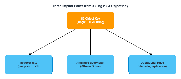
S3 looks deceptively flat. There are no folders, no inodes, no indexes that the user can tune; you write a key, S3 stores the object, you read it back. From the API perspective, the key is just a UTF-8 string with a 1,024-byte limit. From the storage subsystem's perspective, that same string is a routing decision into a partitioned, distributed key-value store, and from any analytics service's perspective, the same string is the only metadata available for partition pruning before you start paying to read bytes.

This is why "key design" is not a stylistic concern. The same key string simultaneously dictates:

Performance. S3 partitions request handling per key prefix. A bucket with one prefix and a million objects under it serves dramatically less throughput than a bucket whose objects are spread across thousands of prefixes — even if the total object count and size are identical.
Queryability. Athena, Redshift Spectrum, EMR, and Glue all rely on path components to skip data. Querying SELECT * FROM logs WHERE day='2026-05-01' is fast if the partition column maps to a directory level, and a full table scan if it does not.
Operations. S3 Lifecycle, Replication, Inventory, and bucket policies all match on prefixes. A flat keyspace with no logical structure leaves you no surface area to apply different rules to different subsets.

In other words, the key is the only "schema" S3 has. Treat it like one.

1.1 What this article covers

This article is a tour through eight concerns, in roughly the order you should think about them when designing a new bucket layout:

How S3 currently partitions request handling (Section 2)
What characters and patterns are safe in keys (Section 3)
How to lay out time-series data (Section 4)
How those layouts integrate with Athena and the Glue Data Catalog (Section 5)
When to switch from catalog partitions to partition projection (Section 6)
How key shape interacts with lifecycle and storage classes (Section 7)
The most common anti-patterns and how to avoid them (Section 8)
How to migrate a bucket whose key design is already wrong (Section 9)

1.2 What this article does not cover

Pricing, cost calculations, or storage-class price comparisons
Comparisons against other object stores (Google Cloud Storage, Azure Blob, MinIO)
The physical layer below S3's key partitioning subsystem
Encryption, access control, and bucket policies — except where they intersect with key design

1.3 The cost of getting it wrong

Before diving into mechanics, it's worth being concrete about what "wrong" looks like in practice. The bills typically come due in four shapes:

Latency. Athena queries that take 30 seconds because partition listing dominates. CloudFront cache misses concentrated on a single hot prefix that returns 503s under load.
Engineering time. Quarterly migrations to peel one team's data out of a shared bucket because the lifecycle rules cannot distinguish them. Every refactor that has to special-case the legacy layout because customers depend on the existing keys.
Lost data. Inadvertent deletion via overly broad lifecycle rules that catch more than intended because the prefix structure is too coarse.
Compliance fire drills. "Show me everything we have for tenant X" answered by a multi-day full-bucket scan instead of a single-prefix list.

None of these show up on day one. They accumulate over the first 18–36 months of a bucket's life and are extraordinarily expensive to undo. The decisions you make in the first week of a new bucket's existence are the ones that determine which side of this curve you end up on.

2. How S3 Partitions Keys (Modern Architecture)

The single most important fact about S3 performance, and the one most frequently misremembered, is the post-2018-07 architecture. Everything else in this article assumes you understand it.

2.1 The pre-2018 model and why randomized prefixes were recommended

For most of S3's first decade, request rate was throttled at the bucket level by a static internal partitioning scheme. Per the original 2018 announcement, a bucket could sustain roughly 100 PUT/LIST/DELETE requests per second and 300 GET requests per second before partitioning kicked in. To get more throughput, customers were instructed to introduce entropy at the start of the key — typically by hashing some part of the key and using the first few hex characters as a prefix. A key like 2018/05/01/event_abc.json would become a3f2/2018/05/01/event_abc.json, deliberately spreading writes across S3's internal partitions.

This guidance is now obsolete. The S3 performance whitepaper states this explicitly: "This guidance supersedes any previous guidance on optimizing performance for Amazon S3. For example, previously Amazon S3 performance guidelines recommended randomizing prefix naming with hashed characters to optimize performance for frequent data retrievals." Randomizing prefixes today actively hurts you because it destroys the lexicographic locality that Athena, Glue, and lifecycle rules all depend on.

2.2 The current model: per-prefix auto-scaling

Since July 17, 2018, S3 automatically scales request capacity per prefix. The headline numbers, copied verbatim from the S3 documentation, are:

3,500 PUT/COPY/POST/DELETE requests per second per partitioned prefix
5,500 GET/HEAD requests per second per partitioned prefix

Two crucial properties follow from this:

There is no limit on the number of prefixes per bucket. You can scale a bucket horizontally by spreading writes across many prefixes. Ten prefixes get you up to 55,000 GETs per second; one hundred prefixes get you up to 550,000.
The scaling is automatic but not instantaneous. When request rate climbs into a new regime, S3 may return HTTP 503 ("Slow Down") responses while it splits the prefix into new internal partitions. The S3 SDKs implement exponential backoff with jitter to absorb this transient.

2.3 What "prefix" actually means

This is the most important conceptual point in the entire article, and the one most often gotten wrong: a "prefix" in the S3 performance sense is not necessarily what you think of as a folder. It is any leading substring of the key, and S3 picks the partitioning point internally based on actual access patterns.

This means three things in practice:

You don't declare prefixes. You write keys, and S3 decides where to split.
Two keys that share a long common prefix will be served by the same internal partition until S3 chooses to split them.
When S3 splits a prefix, it does so transparently. Your application sees only the 503s during the split, not the split itself.

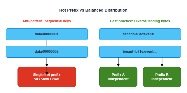
The practical implication: your goal as a key designer is not to manually shard, but to give S3 enough lexicographic spread that auto-partitioning has somewhere to cut. Sequential keys (00000001, 00000002, ...) all share long common prefixes for long stretches, and S3 has nowhere to cut. Diverse keys (a3f2/..., b71e/..., ...) split easily — but at the cost of losing lexicographic locality, which is also valuable.

The modern compromise, covered in Section 4, is to put a high-cardinality dimension early in the key (such as a tenant ID or hashed shard key) when you genuinely need beyond-single-prefix throughput, while keeping a Hive-style time partition layout that Athena understands. For most workloads, the per-prefix limits of 3,500/5,500 are sufficient on their own.

Hot prefix formation: sequential keys vs balanced layout

2.4 When per-prefix limits stop being enough

Most workloads never hit 3,500 writes per second to a single prefix. The ones that do are usually:

High-volume event ingestion (clickstream, IoT telemetry, ad-impression logs)
Aggressive batch loads that compact thousands of small files into one prefix simultaneously
Archival jobs that copy entire S3 inventories from one bucket to another in parallel

For these, you need the key's leading bytes to differ across concurrent writers. The cleanest way to get this is to push a high-cardinality dimension up front — a tenant ID, a region code, or, as a last resort, a hash prefix. Note that this is not the same as the pre-2018 hash-prefix advice: today the goal is operational scalability for known hot prefixes, not a default for every bucket.

2.5 Sharding patterns when you genuinely need them

There are three sharding patterns worth knowing, in increasing order of how aggressive they are about destroying lexicographic locality:

Pattern A: Natural high-cardinality leading segment. If your data is naturally tenant-scoped, region-scoped, or device-scoped, putting that dimension at the start of the key gets you spread for free without any explicit hashing:

tenant=acme/year=2026/month=05/day=06/event_001.json
tenant=globex/year=2026/month=05/day=06/event_002.json

Athena queries that filter by tenant get partition pruning; lifecycle rules can be applied per tenant; and S3's auto-partitioning has thousands of distinct leading bytes to split on. This is the right default for any multi-tenant workload.

Pattern B: Reverse-encoded sequence number. When the only natural key is sequential (database row IDs, Kafka offsets, monotonically increasing sequence numbers), reversing the digits puts the high-cardinality bytes first:

000000007654321  ← original ID (low-cardinality leading bytes)
123456700000000  ← reversed (high-cardinality leading bytes)

S3 still gets a wide spread to partition on, while you preserve the property that two adjacent IDs end up in lexicographically distant places. The downside is that range queries on the original ID become full scans — only do this when range queries are not on the access path.

Pattern C: Hex-prefix sharding. When neither A nor B is available — for instance, you genuinely have a single tenant writing too fast for one prefix — prepend the first one or two hex characters of a hash of some part of the key:

a3/data/2026/05/06/event_001.json
b7/data/2026/05/06/event_002.json
c0/data/2026/05/06/event_003.json
...
ff/data/2026/05/06/event_NNN.json

A two-character hex prefix gives you 256 distinct leading prefixes. This is the modern survivor of the pre-2018 "hash-prefix everything" pattern: use it when you must, never as a default. Athena queries against this layout cannot prune on the hash prefix at all (it's noise), so when you query, you scan all 256 buckets — keep that in mind when picking the prefix length.

Anti-shard pattern. What you should not do is wrap your application in a layer that hashes every key globally. That destroys lexicographic locality for every prefix and breaks Athena, Glue, lifecycle, and replication rule design. Sharding is a targeted tool, not a wholesale architectural choice.

3. Naming Conventions (Allowed Characters, Encoding Pitfalls)

S3 advertises that any UTF-8 string up to 1,024 bytes is a valid key, but this is misleading. The set of keys that work without surprises is much smaller than the set of keys S3 will accept.

3.1 Safe characters

The S3 User Guide partitions characters into three groups: safe, special-handling, and avoid. Safe characters do not need to be percent-encoded, do not collide with URL or shell parsing, and round-trip through every SDK and tool the AWS ecosystem ships:

0-9 a-z A-Z (ASCII alphanumerics)
! - _ . * ' ( ) (a fixed set of seven safe punctuation characters)
/ (the path separator — always safe)

If your key generator only produces characters from these sets, you will not run into encoding issues. Most production layouts should aim for this.

3.2 Characters that require special handling

The following characters are technically allowed but trigger percent-encoding in URLs and may need extra care in scripts: space, & $ @ = ; : + , ?. Spaces in particular are a frequent source of bugs because they survive S3 itself but then break shell pipelines and CSV manifests.

3.3 Characters to avoid

ASCII control characters (values 0–31 and 127): some SDKs cannot serialize them in XML responses, and S3 itself recommends URL-encoding the response when keys contain them
\ { } ^ % " < > [ ] # | ~: these are reserved in URLs, RFC paths, or both
ASCII values 0 through 10 specifically: XML 1.0 parsers cannot represent these, and ListObjects / ListObjectsV2 will fail to encode them unless you explicitly request EncodingType=url in the response

3.4 Period-only path segments

The S3 User Guide explicitly warns against keys containing . or .. as path segments. While S3 stores these literally, downstream tools normalize them aggressively:

Many client libraries collapse folder/./file.txt to folder/file.txt
.. is interpreted as parent-traversal in shells and some SDKs
The CLI may refuse to upload or list paths containing these segments

The fix is simple: never use a single dot or double dot as a complete path segment. They are fine inside a segment (config.v2.json) but never alone.

3.5 The "soap" gotcha

Object key names with the value soap are not supported for virtual-hosted-style requests. This is a holdover from S3's SOAP API era. If a key contains soap as a complete segment, requests must use path-style URLs. Most modern SDKs handle this transparently, but it surfaces as a confusing 400 in old code paths.

3.6 Length, case, and Unicode

The key length limit is 1,024 bytes, not characters. Multi-byte UTF-8 sequences (most non-ASCII text) consume 2–4 bytes per character. A purely ASCII key has 1,024 characters of headroom; a Japanese-language key has roughly 340.
Object keys are case-sensitive. Photos/2026.jpg and photos/2026.jpg are different objects.
S3 stores keys as the literal byte sequence you upload. It does not normalize Unicode. If half your producers send NFC and half send NFD, you will end up with two distinct keys for what looks like the same name. Pick one normalization form and enforce it at the producer.

3.7 A reusable naming template

The conventions above can be summarized as a single naming template that has worked well across many production deployments:

{prefix-key=value}/{prefix-key=value}/{ingest-time}/{producer-id}_{sequence}.{ext}

All segments lowercase
Letters, digits, and _ - . only
Time uses ISO-8601 components (year=YYYY/month=MM/day=DD) — see Section 4
The final filename component is unique enough to avoid accidental collisions across producers
Total key length stays well under 256 bytes, leaving headroom for metadata systems that limit key length more aggressively than S3

4. Time-Series Layouts (Hive Style vs Project Style)

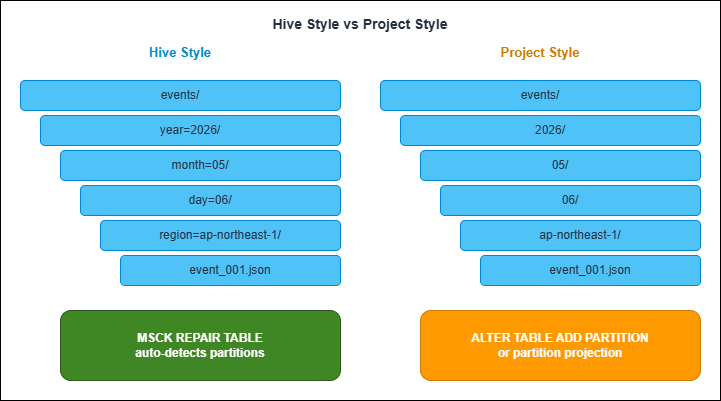
Most data lakes are time-partitioned. The two ways to encode time in the key are not equivalent — they trade off different operational properties.

4.1 Hive style

Hive-style partitioning encodes both the partition column name and its value into the path:

s3://bucket/events/year=2026/month=05/day=06/region=ap-northeast-1/event_001.json

Athena, Glue, EMR, and most Apache-ecosystem tools recognize this format natively. Running MSCK REPAIR TABLE against an external table backed by this prefix layout discovers all partitions automatically.

4.2 Project style

Project-style partitioning omits the column name and only writes the value:

s3://bucket/events/2026/05/06/ap-northeast-1/event_001.json

This is the format used by Amazon CloudTrail, Amazon Data Firehose (with default settings), VPC Flow Logs, and most AWS service-emitted logs. Athena does not auto-detect partitions in this format — you must either declare the columns manually with ALTER TABLE ADD PARTITION, configure partition projection (Section 6), or run a Glue Crawler against the bucket.

4.3 Comparison

Hive style vs Project style time-partition layout

* You can sort the table by clicking on the column name.

Aspect	Hive Style (`year=YYYY/`)	Project Style (`YYYY/`)
Athena partition discovery	Automatic via `MSCK REPAIR TABLE`	Manual via `ALTER TABLE ADD PARTITION` or projection
Glue Crawler compatibility	Auto-detects partition columns	Requires per-bucket configuration
Path length	Longer (column names included)	Shorter
Human readability	High (self-describing)	Lower (positional only)
AWS service emitter default	Rare (must opt in via Firehose dynamic partitioning)	Common (CloudTrail, Flow Logs, native Firehose)
Refactor cost when adding a new column	Low (insert a new `key=value` segment)	High (changes positional meaning)
Risk of column-position drift	Low	High (especially when teams change ordering)

4.4 Choosing between them

The decision rule that has held up across many migrations:

Use Hive style when you control the writer. It gives you cheaper partition management, safer schema evolution, and free Athena partition discovery. The longer keys are a price worth paying.
Use project style when AWS emits the data for you. Don't fight the format — instead, use partition projection (Section 6) to teach Athena the layout without rewriting the keys.
Never mix them in the same bucket. A bucket with year=2026/... for some objects and 2026/... for others is unqueryable as a single table.

4.5 Granularity choice

Independent of style, you also pick how deep the time hierarchy goes:

year=2026/                              ← yearly
year=2026/month=05/                     ← monthly
year=2026/month=05/day=06/              ← daily
year=2026/month=05/day=06/hour=14/      ← hourly
year=2026/month=05/day=06/hour=14/min=30/ ← per-minute

The right depth is determined by query patterns, not data volume. If most queries filter by day, partition by day. If queries are evenly distributed across hours, partition by hour. A common mistake is to partition by minute "just in case" — this multiplies partition count by 60 with no query benefit, and pushes you toward Glue Catalog limits much faster than necessary.

5. Athena and Glue Catalog Integration

Once data is laid out, Athena needs to know about the partitions before queries can prune them. There are three distinct mechanisms, and choosing among them is one of the higher-leverage decisions in this entire article.

5.1 MSCK REPAIR TABLE

MSCK REPAIR TABLE scans the S3 prefix backing a table and adds any new Hive-style partitions it finds to the Glue Data Catalog. It is the canonical way to bootstrap or refresh a Hive-partitioned table.

MSCK REPAIR TABLE events;

What it does well:

Zero configuration: works on any Hive-style layout
One command catches up an arbitrary backlog of new partitions

What it does poorly:

It only adds partitions; it never removes stale ones. If you delete partitions in S3, run ALTER TABLE ... DROP PARTITION separately
It silently fails on partition values containing colons (:), which is exactly what you get if you encode timestamps naively
It does not pick up partition columns whose name starts with an underscore
It can hit memory limits on tables with more than approximately 100,000 partitions

For tables with growing partition counts, MSCK REPAIR TABLE is a starter solution, not an end state.

5.2 ALTER TABLE ADD PARTITION

For project-style layouts and any layout MSCK REPAIR TABLE does not handle (such as keys with colons), you declare partitions explicitly:

ALTER TABLE flow_logs
ADD PARTITION (year='2026', month='05', day='06')
LOCATION 's3://my-flow-logs/AWSLogs/123456789012/vpcflowlogs/ap-northeast-1/2026/05/06/';

This is precise but verbose. In production, it is almost always wrapped in automation (a Lambda triggered by S3 events, or a scheduled job that adds tomorrow's partition before midnight UTC). The mechanical generation of ADD PARTITION statements is what partition projection (Section 6) ultimately replaces.

5.3 Glue Crawlers

A Glue Crawler scans an S3 prefix on a schedule, infers schema and partition columns, and writes them to the Glue Data Catalog. For Hive-style layouts, it auto-detects partition keys from the key=value segments. For project-style, you configure a custom classifier that maps positional segments to column names.

Crawlers absorb the schema-management problem at the cost of a periodic scan that grows with bucket size. For tables with bounded growth and infrequent schema changes they are convenient. For tables that grow continuously (most data lakes) they become slower over time and eventually need to be replaced with partition projection.

5.4 The progression most teams follow

A typical lifecycle for a partitioned table:

Day 1: Hive-style layout, MSCK REPAIR TABLE after initial load
Day 30: Add a daily Lambda that runs MSCK REPAIR TABLE or ALTER TABLE ADD PARTITION for the previous day
Day 365: Partition count crosses 10,000+, queries spend a noticeable fraction of their time on partition listing, switch to partition projection (Section 6)
Day 1000: The catalog is read-only metadata; all partition resolution happens at query time

The earlier you anticipate this trajectory, the less rework you do.

5.5 Monitoring partition growth

The transition from "the catalog is fine" to "the catalog is the bottleneck" is gradual and often invisible. By the time queries are slow, the cost of switching to projection is no longer just an architecture change — it's a refactor of every consumer that has assumed the catalog is the source of truth.

Two signals worth tracking:

Partition count per table. Glue Catalog has a soft limit of 10 million partitions per table, but query planning latency starts to hurt well before that. A SHOW PARTITIONS my_table query that takes more than a few seconds is your warning sign.
Query planning time. Athena emits planning time as a separate metric from execution time. If planning time grows linearly with partition count while execution time stays flat, you've hit the partition listing ceiling.

Both signals are visible in CloudWatch metrics and the Athena query history. A small dashboard checking partition count growth weekly catches the transition months before users notice.

6. Partition Projection

When the partition count grows enough that partition listing dominates query latency, partition projection is the standard answer. Instead of materializing every partition in the Glue Catalog, you tell Athena how to compute partitions from the WHERE clause at query time.

6.1 When to use it

Partition projection is the right tool when any of these apply:

The table has more than ~10,000 partitions
The table is laid out in project style and you don't want to pre-register every partition
Partition columns are time-derived (year, month, day, hour)
Partition values follow a regular grammar (a small enum, an integer range, a date range)
The query pattern always includes a WHERE clause on the partition columns

It is the wrong tool when:

Partition values are unpredictable strings with no enumerable structure (use catalog partitions or an injected projection — see 6.4)
Queries frequently scan all partitions (projection's cost model breaks down without a WHERE clause)

6.2 The four projection types

Athena supports exactly four projection types. Choose based on how the column's values are generated:

integer — for columns whose values are consecutive integers within a known range. Limited to the Java signed long range (-2^63 to 2^63-1). Good for sequence numbers, day-of-year encodings, and similar.
date — for columns whose values are dates or timestamps within a known range. Supports a format (Java DateTimeFormatter pattern), interval, and interval.unit. The range can be open-ended via the NOW keyword.
enum — for columns whose values are members of a small, fixed set. Athena recommends keeping enum projections to a few dozen values or less; query planning slows down as the value count grows, and the Glue Catalog's table parameter size limits cap how many enum values you can store.
injected — for columns whose cardinality is too high to enumerate (user IDs, device IDs, tenant codes). Requires every query to include a static equality predicate (WHERE user_id = '...') on the projected column; otherwise Athena rejects the query.

6.3 A worked example: a Hive-style time-partitioned table

The TBLPROPERTIES block looks like this:

CREATE EXTERNAL TABLE events (
  event_id string,
  payload string
)
PARTITIONED BY (year int, month int, day int)
STORED AS PARQUET
LOCATION 's3://my-events-bucket/events/'
TBLPROPERTIES (
  'projection.enabled'                = 'true',
  'projection.year.type'              = 'integer',
  'projection.year.range'             = '2024,2030',
  'projection.month.type'             = 'integer',
  'projection.month.range'            = '1,12',
  'projection.month.digits'           = '2',
  'projection.day.type'               = 'integer',
  'projection.day.range'              = '1,31',
  'projection.day.digits'             = '2',
  'storage.location.template'         = 's3://my-events-bucket/events/year=${year}/month=${month}/day=${day}/'
);

A query like WHERE year=2026 AND month=5 AND day=6 resolves to exactly one path. A query like WHERE year=2026 AND month=5 resolves to 31 paths. Athena never lists the bucket — it computes the prefixes from the projection and asks S3 only for the objects under those prefixes.

6.4 Injected projection for high-cardinality keys

For tenant-style data — millions of unique tenant IDs in the partition key — the injected type is the only sensible choice:

PARTITIONED BY (tenant_id string, day string)
TBLPROPERTIES (
  'projection.enabled'        = 'true',
  'projection.tenant_id.type' = 'injected',
  'projection.day.type'       = 'date',
  'projection.day.format'     = 'yyyy-MM-dd',
  'projection.day.range'      = '2024-01-01,NOW',
  'storage.location.template' = 's3://multi-tenant-data/tenant=${tenant_id}/day=${day}/'
);

Every query against this table must include a static equality on tenant_id — for example, WHERE tenant_id = 'acme' AND day BETWEEN '2026-05-01' AND '2026-05-06'. This is exactly the access pattern most multi-tenant analytics workloads have, and the constraint forces query authors to be explicit about which tenant they're scanning, which is also good for cost predictability.

6.5 Partition Projection Calculator tool

Computing the cartesian product of projected partitions, previewing the resulting S3 paths, and exporting the TBLPROPERTIES block is mechanical but error-prone — small mistakes in the format string or range produce empty results without a clear error. The site includes a client-side tool that does this work in the browser:

Athena Partition Projection Calculator - Partition Count and Path Preview Tool
You enter a storage.location.template and the type of each projection column; the tool returns the per-column cardinality, the cartesian-product total partition count with a severity rating, ten sample paths (first five and last five), and the full TBLPROPERTIES block as YAML or as an AWS::Glue::Table CloudFormation snippet. It is particularly useful for sizing decisions — if the calculator returns "Excessive (more than 1 million partitions)," that is a clear signal to coarsen the granularity before the table goes to production.

6.6 Common partition projection mistakes

Five mistakes I see often enough to flag in any partition projection review:

Forgetting projection.enabled = 'true'. Without this top-level flag, every other projection.* property is ignored. Athena falls back to catalog-based partitions silently — your queries still work, just slowly. Always confirm the flag is set when troubleshooting "projection not working."
Format string drift. 'projection.month.format' = 'MM' and 'projection.month.format' = 'M' are different. With 'MM' Athena expects two digits (05); with 'M' it expects one or more (5). If your data is written with 05 but the projection is configured for M, queries return empty results. Match the actual on-disk format byte for byte.
Range covering the future too generously. A range of 2020-01-01,NOW is fine; a range of 2020,2099 is also fine for years. But a range of 1,1000000000 for an integer column will cause Athena to materialize a billion-row partition list at query plan time even when the WHERE clause narrows it. Bound the range to what's actually possible.
Not using NOW for date ranges that grow. Hard-coding the upper bound (2024-01-01,2025-12-31) means you have to update the table every year. The NOW literal is evaluated at query time and lets the projection grow without intervention.
Mixing enum with high cardinality. Glue table parameter size limits and growing query-plan latency together cap how many enum values you can store; about a few dozen is the practical ceiling. If your column has hundreds or thousands of distinct values, switch to injected and accept the WHERE-clause requirement.

7. Lifecycle and Storage Class Considerations

S3 Lifecycle rules and storage-class transitions both match on prefixes. Key design therefore directly shapes the surface area available for these rules.

7.1 Lifecycle rule prefix matching

A Lifecycle rule applies to objects whose key matches an optional prefix and (since 2019) optional tags. A bucket with a flat keyspace exposes only one knob: "all objects, X days." A bucket with a structured prefix layout exposes one knob per prefix: "logs/raw older than 30 days transition to Glacier Instant Retrieval, logs/processed older than 7 days expire."

The implication for key design: if any subset of objects in a bucket needs different lifecycle treatment than the rest, that subset should live under its own prefix. Trying to retrofit a structured prefix later is a copy-and-delete operation across the entire bucket (Section 9).

7.2 Time partitions and aging policies

Time-partitioned layouts make age-based lifecycle rules trivial — every partition above a certain age is below a certain prefix. A rule like "transition to Glacier after the partition is 90 days old" maps directly to lifecycle rules on year=2025/month=01/, year=2025/month=02/, and so on, without any object-tag scanning.

7.3 Replication selectivity

S3 Replication rules also use prefix matching. A common pattern in regulated industries is to replicate only certain prefixes cross-region — for example, replicating pii/ to a region with stricter sovereignty rules while leaving logs/ in the original region. If everything is mixed under a single flat prefix, you cannot do this without a per-object tag scan; with a structured layout, you write one rule and it just works.

The same is true in reverse for selective non-replication: a temp/ prefix that is excluded from replication entirely (because it's intermediate compute output that doesn't need to survive a regional failure) is much cheaper to operate than tagging every temp object individually.

7.4 What to read next

Detailed lifecycle and storage-class strategy is its own topic and not the subject of this article — see the official S3 documentation linked in the References section. The key takeaway here is that lifecycle and replication rules are downstream consumers of your key design. If the keys are well-structured, every other rule writes itself; if they're not, every rule becomes a workaround.

8. Anti-Patterns

The patterns below are common enough that a short tour through them will likely flag at least one issue in any bucket that has been around for a few years.

8.1 Sequential numeric prefixes

The pattern: bucket/data/0000001/object, bucket/data/0000002/object, ... — produced by counters, database IDs, or "files numbered in order."

The problem: every key shares the prefix bucket/data/000000. S3 cannot easily auto-partition because the leading bytes are nearly identical. As traffic grows, this prefix becomes hot and you start seeing 503s.

The fix: either reverse the numeric component (so 0000001 becomes 1000000, spreading high-cardinality digits to the front), prepend a hash of the ID, or rethink whether the sequence number needs to be the first segment at all. Putting an entity type or tenant ID first usually fixes it.

8.2 Timestamp-leading keys

The pattern: bucket/2026/05/06/14/30/45/event.json, with the time at the very start of the key.

The problem: at any single instant, every concurrent writer is writing to the same prefix. If you write 10,000 events per second, you have 10,000 writes per second concentrated on one minute-level prefix.

The fix: put a high-cardinality dimension before the time component, or shift the time granularity coarser so the prefix splits more often. Keys like bucket/tenant=abc/2026/05/06/event.json solve the immediate problem because the tenant ID provides spread.

8.3 Single fixed coordination keys

The pattern: an object at a fixed key like bucket/state/lock.json or bucket/queue/head that the application reads, modifies, and writes back as a coordination primitive.

The problem: S3 is not a coordination primitive. A single hot key against the storage layer caps at a few thousand requests per second, doesn't have multi-writer semantics, and provides no atomicity guarantees beyond per-object writes.

The fix: use the right tool. DynamoDB conditional writes, S3 Conditional Writes for the simple cases (since 2024-11), or a dedicated coordination service (Step Functions, EventBridge Pipes, SQS) is almost always correct.

8.4 The "tail of the bucket" hot spot

The pattern: an index.html or latest.json at a fixed key that every reader requests (often via CloudFront).

The problem: in itself this is fine — CloudFront absorbs read traffic. But the same pattern at the head of every prefix (year=2026/index.html, year=2026/month=05/index.html, ...) and uncached creates many small hot spots.

The fix: cache hot read paths in CloudFront with a sensible TTL. If a TTL is incompatible with the use case, the data probably belongs in DynamoDB, not S3.

8.5 Mixing partition styles

The pattern: a bucket containing both events/year=2026/month=05/... and events/2026/05/... because two teams added their data at different times.

The problem: neither pattern alone is queryable as a single Athena table. The bucket can only be queried as two separate tables, or by an expensive ETL pass that homogenizes the layout.

The fix: standardize at the bucket level. The prefix-design contract for the bucket should be documented somewhere a new team can find it before they start writing, not after.

8.6 The "magic" delimiter

The pattern: keys like bucket/tenant_abc__2026__05__06__event.json that encode multiple dimensions into a single segment using a delimiter that isn't /.

The problem: nothing on the S3 side can use these substructure dimensions for partitioning, lifecycle, or queries. Athena and Glue can only see the segment as a single string column.

The fix: make each dimension its own path segment. tenant=abc/year=2026/month=05/day=06/event.json is longer but lets every other AWS service operate on it.

8.7 Unicode normalization mismatch

The pattern: producers running on different operating systems write keys containing non-ASCII characters using different Unicode normalization forms — typically NFC on most systems but NFD on macOS for filenames containing diacritics.

The problem: S3 stores the byte sequence verbatim and does not normalize. The string café written as NFC (U+0063 U+0061 U+0066 U+00E9, 4 code points) and as NFD (U+0063 U+0061 U+0066 U+0065 U+0301, 5 code points) are different keys. Lookups, deduplication, and HEAD checks all fail when one writer expects what the other produced.

The fix: enforce one normalization form at the producer. NFC is the right default for almost everyone — it's the W3C-recommended form, what most browsers send, and the most compact representation. Add a normalization step before any code path that constructs an S3 key, and reject any non-normalized key at the bucket boundary if you must accept user input.

8.8 Versioning hidden in the key name

The pattern: keys like bucket/data/2026/05/06/event_v1.json, event_v2.json, event_v3.json — version numbers baked into the key.

The problem: the bucket already has a versioning feature. Encoding versions in the key duplicates the responsibility, makes "fetch the latest version" a LIST operation instead of a single GET, and breaks Athena queries that expect a stable filename per partition.

The fix: enable S3 Versioning on the bucket and let S3 manage version history. Use GET with no versionId to fetch the current version; use ListObjectVersions when you actually need history. Reserve key-name versioning for the rare cases where you genuinely need parallel versions visible to consumers (an index.json and a previous-index.json for a static rollback path, for example).

9. Migration: Re-keying Strategies

Eventually you discover that an existing bucket has the wrong layout. There are three ways to fix it, varying by data volume and downtime tolerance.

9.1 Approach A: S3 Batch Operations Copy job

For one-shot migrations of any size, S3 Batch Operations is the standard tool. You provide a manifest (CSV or S3 Inventory report) listing every source object, plus a Lambda function or a built-in copy job that maps source keys to destination keys. Batch Operations then iterates through the manifest, parallelizing the copy across thousands of workers.

The shape of the workflow:

aws s3control create-job \
  --account-id 123456789012 \
  --operation '{
    "S3PutObjectCopy": {
      "TargetResource": "arn:aws:s3:::dst-bucket",
      "TargetKeyPrefix": ""
    }
  }' \
  --manifest '{
    "Spec": {
      "Format": "S3InventoryReport_CSV_20211130",
      "Fields": ["Bucket","Key"]
    },
    "Location": {
      "ObjectArn": "arn:aws:s3:::inventory-bucket/manifest.json",
      "ETag": "60e460c9d1046e73f7dde5043ac3ae85"
    }
  }' \
  --report '{
    "Bucket":"arn:aws:s3:::report-bucket",
    "Format":"Report_CSV_20180820",
    "Enabled":true,
    "Prefix":"job-reports/",
    "ReportScope":"AllTasks"
  }' \
  --priority 10 \
  --role-arn arn:aws:iam::123456789012:role/S3BatchOperationsRole \
  --region us-east-1

For non-trivial key transformations (anything beyond a fixed prefix replacement), the operation should be LambdaInvoke instead of S3PutObjectCopy, with a Lambda that computes the destination key from the source key.

In standard general-purpose S3 buckets there is no native rename operation. Every "rename" is a copy followed by a delete. The native RenameObject API exists only for directory buckets in the S3 Express One Zone storage class.

9.2 Approach B: Event-driven key-rewriting Lambda

For continuous migration where the source bucket keeps receiving writes, the standard mechanism is an event-driven rewrite pipeline: configure S3 Event Notifications (or an EventBridge rule) on the source bucket to trigger a Lambda function that copies each new object to the destination bucket with the rewritten key. S3 Replication on its own is not sufficient because it preserves the source key path apart from an optional destination prefix and cannot perform arbitrary key rewrites.

This approach lets you do a "double-write" period: producers continue writing to the old bucket; the rewrite pipeline mirrors each new object to the new bucket under the new layout; consumers gradually move to the new bucket; eventually the old bucket is drained.

9.3 Approach C: Side-by-side parallel write

When you control the producers and the cost of running both layouts in parallel for a transition window is acceptable, the simplest migration is no migration at all: have producers write to both layouts simultaneously for a window long enough to cover the data retention period of all consumers, then cut consumers over and turn off the old layout.

This avoids the manifest-and-copy machinery entirely. It is the only approach that works cleanly for tables that include columns derived from the key itself (the destination layout would have a different column derivation).

9.4 A cutover playbook for the data side

The mechanical copy is rarely the hard part. The cutover — the moment consumers stop reading the old layout and start reading the new — is where things tend to break. The playbook that has worked across many migrations:

Inventory. Generate a current S3 Inventory report on the source bucket. Capture object count and total size by prefix. This is the baseline you measure progress against.
Build the new bucket empty. Configure the destination bucket with the new layout's lifecycle, replication, and event notification rules from the start. Do not retrofit them after the data is in.
Replay history. Run the S3 Batch Operations Copy job (or your equivalent) on a snapshot. Verify the destination object count and total size match the source minus expected losses (objects deleted between snapshot and copy).
Start dual-write. Update producers to write to both buckets. Monitor for divergence between the two using a periodic diff job — for a busy bucket, even a small bug in the new code path can produce silent inconsistency.
Cut over consumers gradually. Move the lowest-risk consumer first (a daily batch report, an internal dashboard). Watch for a week. Move the next-highest. Production-critical consumers move last.
Drain the old bucket. Once no consumer depends on the old layout, set a lifecycle rule to expire old objects on a long timeline (60–90 days), then delete the bucket. Don't shortcut this — once it's gone, recovery is forensic.

For tables registered in the Glue Data Catalog, every step above has a corresponding catalog action: a parallel table pointing at the new location, a switch of the canonical table name, a backfill of partitions on the new table. Coordinate those changes with the consumer migration, not after.

9.5 A migration checklist

Before any of the three approaches:

Inventory: run an S3 Inventory report on the source bucket to know exactly how much you're migrating
Lifecycle: check whether the source bucket has lifecycle rules that will expire objects mid-migration
Versioning: if the source bucket is versioned, decide whether to migrate all versions or only the current ones
Replication: if the source bucket is already a replication target, plan how to handle the in-flight chain
Glue Catalog: any tables backed by the source location need updated LOCATION clauses
Lambda triggers / EventBridge rules: any S3 event notifications need to be re-pointed
Access policies: bucket policies and IAM policies referencing prefixes need to be updated for the new layout

The catalog and downstream rule updates are usually where things go wrong, not the data movement itself.

10. Summary

S3 object keys are the only schema S3 has, and that schema is permanent in the same way a primary key is permanent — every other operational and analytical decision is built on top of it. The decisions that pay the most compounding interest:

Treat the post-2018 per-prefix scaling (3,500 writes / 5,500 reads per partitioned prefix) as the ground truth. Don't randomize prefixes by default; let auto-partitioning do its job.
Pick a naming convention with safe characters, a single Unicode normalization form, and never use . or .. as a complete path segment.
For controllable producers, prefer Hive-style time partitioning. For AWS-emitted logs, use partition projection rather than rewriting the layout.
Plan for the catalog-to-projection transition before you cross 10,000 partitions.
Anti-patterns (sequential prefixes, timestamp-leading keys, single coordination keys) are easy to spot in code review; train the team to flag them early.
When you do need to migrate, S3 Batch Operations with a Lambda is the most flexible tool. Copy semantics, not rename — this is also true at scale.

The thing that distinguishes a bucket that ages well from one that doesn't is rarely a single dramatic decision. It's the accumulation of small, consistent constraints applied at the moment of design and never violated afterward.